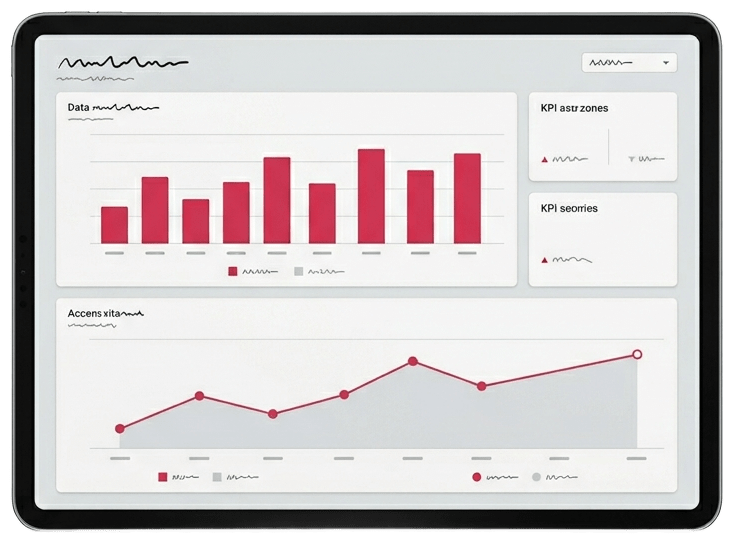
Market research, survey methodology and their practical application — from research problem to results report.
Dr. Paul Marx · QUESTIONSTAR
Slide 01 · 261
QUESTIONSTAR
Build · Survey · Analyze · Report
1
Chapter 1 · Introductory Course
Principles of Survey Research
Market research, survey methodology and their practical application — from research problem to results report.
Dr. Paul Marx · QUESTIONSTAR
Slide 01 · 261
QUESTIONSTAR
Build · Survey · Analyze · Report
Chapter 1 · Introductory Course
Principles of Survey Research
Market research, survey methodology and their practical application — from research problem to results report.
Dr. Paul Marx · QUESTIONSTAR
Slide 01 · 261
QUESTIONSTAR
Build · Survey · Analyze · Report
Chapter 1 · Introductory Course
Principles of Survey Research
Methodologically sound. Practically applicable.
Market research, survey methodology and their practical application — from research problem to results report.
Dr. Paul Marx · QUESTIONSTAR
Chapter 1 · IntroductionTable of Contents
Contents
01Introduction
1.1Market Research and Survey
1.2Types of Market Research
02Survey: Measurement and Scaling
2.1Introduction
2.2Comparative Scales
2.3Non-Comparative Scales
2.4Latent Constructs
2.5Reliability and Validity
03Questionnaire
3.1Asking Questions
3.2Overcoming Inability to Answer
3.3Overcoming Unwillingness to Answer
3.4Increasing Willingness of Respondents
3.5Determining the Order of Questions
3.6What's Next?
04Sampling
4.1Non-probability Sampling
4.2Probability Sampling
4.3Choosing Non-probability vs. Probability Sampling
4.4Sample Size
05Data Analysis: A Concise Overview of Statistical Techniques
5.1Descriptive Statistics:Organizing and Presenting Data
5.1.1Organizing Qualitative Data
5.1.2Organizing Quantitative Data
5.1.3Summarizing Data Numerically
5.1.4Cross-Tabulations
5.2Inferential Statistics:Can the results be generalized to the population?
5.2.1Hypothesis Testing
5.2.2Strength of a Relationship in Cross-Tabulation
5.2.3Relationship between Two (Ratio Scaled) Variables
06Advanced Techniques of Market Analysis: Some Useful Concepts
6.1Conjoint Analysis
6.2Market Simulations
6.3Segmentation
6.4Perceptual Positioning Maps
07Reporting Results
QUESTIONSTAR · Dr. Paul Marx02 / 274
Chapter 1Section Overview
1
Chapter
Introduction
1.1Market Research and Survey
1.2Types of Market Research
QUESTIONSTAR · Dr. Paul Marx03 / 274
Chapter 1 · IntroductionSection Overview
1
Chapter
Introduction
1.1Market Research and Survey
1.2Types of Market Research
QUESTIONSTAR · Dr. Paul Marx04 / 274
1.1 · Market Research and SurveyDefinitions
What is Research?
Research is
All systematic endeavors and efforts to acquire new knowledge for science or industry.
— Encyclopedia
Research is
The search for and collection of information and ideas in response to a specific question.
— Practical definition
QUESTIONSTAR · Dr. Paul Marx05 / 274
1.1 · Market Research and SurveyDefinition
Survey
Survey
A survey is one of the most popular methods of collecting primary data, in which the researcher interacts with respondents to obtain information about people's attitudes, opinions, knowledge and behaviors.
1Attitudes & Opinions — how people think and judge
2Knowledge — what people know and understand
3Behaviors — what people actually do
QUESTIONSTAR · Dr. Paul Marx06 / 274
1.1 · Market Research and SurveyUnderstanding the Problem
Market Research
Decision MakerDecision ProblemResearcherDissatisfied customersDeclining market shareFalling salesLow trafficAbove WaterVisible and measurable symptomsBorderline performance of the sales teamPoor delivery serviceInadequate product qualityUnethical treatment of customersPoor imageBelow WaterThe actual business or decision problem
QUESTIONSTAR · Dr. Paul Marx07 / 274
1.1 · Market Research and SurveyFields of Application
Practical Application of Surveys
Discipline
Application
Sociology and Political Science
Opinion research, identifying the attitudes of population groups toward socially significant phenomena, events and facts; election research (e.g. the "Sunday question"), …
Psychology
Personality tests, intelligence tests, identifying individual strengths and weaknesses, psychological stability, cognitive disorders, social influences, …
Results have no practical value if the research problem is only vaguely defined.
The plan must be set in advance, yet flexible — so that necessary adjustments can be built in.
This phase is very costly and very error-prone.
The choice of data analysis method depends essentially on the type of research.
Present actionable key findings rather than overwhelming statistical methods.
QUESTIONSTAR · Dr. Paul Marx09 / 274
1.1 · Market Research and SurveyLimits of Market Research
When should you not start market research projects?
Case
Comment
Vague objectives
When managers cannot agree on what information they need to make a decision. Market research only helps when it investigates a concrete question.
Fixed stance
When the decision has already been made and the study is only meant to "rubber-stamp" a preconceived plan.
Too late
When results are provided too late to still influence the decision.
Poor timing
When a product is in its decline phase, there is little point in researching new product variations.
Insufficient resources
It is not worthwhile to set up a quantitative study as long as no statistically significant sample is feasible — or when the finances are not enough to implement the resulting decisions.
Costs outweigh benefits
The expected value of information should exceed the costs of data collection and analysis.
Results not actionable
When, for example, psychographic characteristics are used that do not help in making concrete decisions.
Information not needed
When decision-relevant information is already available.
QUESTIONSTAR · Dr. Paul Marx10 / 274
Chapter 1 · IntroductionSection Overview
1
Chapter
Introduction
1.1Market Research and Survey
1.2Types of Market Research
QUESTIONSTAR · Dr. Paul Marx11 / 274
1.2 · Types of Market ResearchThree classifying criteria
Types of Market Research
Criterion 1
By Objectives
Exploratoryalso diagnostic
Descriptive
Causalalso predictive, experimental
Criterion 2
By Data Source
Primarydata collected yourself
Secondarydata already available
Criterion 3
By Methodology
Qualitativeunderstand
Quantitativemeasure
QUESTIONSTAR · Dr. Paul Marx12 / 274
1.2 · Types of Market ResearchBy Research Objectives
Market Research by Objectives
Uncertainty shapes the type of market research
Uncertain
Certain
Low clarity
Exploratory
also diagnostic
Problem not yet precisely defined; hypotheses are formed.
Analyzing data and actions to understand problems better
What reasons might lie behind the declining customer satisfaction?
What keeps first-time buyers from buying again?
Medium clarity
Descriptive
Phenomena are systematically described and measured.
Collecting and presenting facts: who, what, when, where, how?
What does the historical sales trend in the industry look like?
Allows comparison of the differences between objects; zero point arbitrary
Temperature (Fahrenheit, Celsius)
Attitudes, opinions, purchase intention, customer satisfaction, index numbers
Range, average, standard deviation
Product-moment correlation (Pearson's r), t-tests, ANOVA, regression and factor analysis
Ratio Scale
Zero point is uniquely fixed; allows comparison of both the distances between measured values and their ratios
Length, weight, time, money
Age, revenue, income, costs, market share
Geometric mean, harmonic mean
Coefficient of variation
QUESTIONSTAR · Dr. Paul Marx23 / 274
2.1 · IntroductionOverview
Classification of Scaling Techniques
Root
Scaling
Comparative Scales
Objects are compared directly with one another
Paired ComparisonRank Order ScalingConstant Sum ScalingQ-Sort Scaling & others
Non-Comparative Scales
Each object is judged in isolation
Continuous Rating Scales
Itemized Rating Scales
Likert ScaleSemantic DifferentialStapel Scale
QUESTIONSTAR · Dr. Paul Marx24 / 274
2.1 · IntroductionComparison
Comparison of Scaling Techniques
Direct
Comparative Scales
The measured value of an object results from the direct comparison with another object.
Data can only be interpreted as relative positions — ordinal ordinal level of measurement only (rank order).
Isolated
Non-Comparative Scales
Each object is judged in isolation — that is, independently of other objects.
Measurement results are usually treated as intervalscaled or metric.
The choice between the scaling techniques depends on:
Nature of the research questionVariability of the measured value in the populationMethods of data analysis
QUESTIONSTAR · Dr. Paul Marx25 / 274
Chapter 1 · Part 2Section Overview
2
Part
Survey: Measurement and Scaling
2.1Introduction
2.2Comparative Scales
2.3Non-Comparative Scales
2.4Latent Constructs
2.5Reliability and Validity
QUESTIONSTAR · Dr. Paul Marx26 / 274
2.2 · Comparative ScalesFocus
Classification of Scaling Techniques
Root
Scaling
Comparative Scales
Objects are compared directly with one another
Paired ComparisonRank Order ScalingConstant Sum ScalingQ-Sort Scaling & others
Non-Comparative Scales
Each object is judged in isolation
Continuous Rating Scales
Itemized Rating Scales
Likert ScaleSemantic DifferentialStapel Scale
QUESTIONSTAR · Dr. Paul Marx27 / 274
2.2 · Comparative ScalesAssessment
Pros-and-Cons of Comparative Scales
+
Pros
Small differences between objects can be registered
The same known reference points for all respondents
Easy to understand and use
Require fewer theoretical assumptions
Tend to reduce halo and carryover effects
−
Cons
Only ordinal or rank-order level of measurement → limited choice of statistical methods for data analysis
Data can only be interpreted as relative positions
Impossible to generalize beyond the set of objects rated
QUESTIONSTAR · Dr. Paul Marx28 / 274
2.2 · Comparative ScalesMethod
Comparative Scales: Paired Comparison
i
Paired Comparison
For each pair of two objects, respondents select the one that in their opinion best fulfills a given criterion.
Below you are presented with ten pairs of beer brands. In each pair, please select the beer you would rather buy.
Warsteiner
Köstritzer
Oettinger
Becks
Paulaner
Warsteiner
←
←
↑
←
Köstritzer
↑
←
↑
←
Oettinger
↑
↑
↑
↑
Becks
←
←
←
←
Paulaner
↑
↑
←
↑
# times preferred
3
2
0
4
1
QUESTIONSTAR · Dr. Paul Marx29 / 274
2.2 · Comparative ScalesPractical Example
Comparative Scales: Paired Comparison
If these two computers were equal in everything else — which would you prefer?
Pair 3 of 10
Computer on the left
1 TB SSD
128 GB RAM
Computer on the right
2 TB SSD
36 GB RAM
Clearly prefer leftSomewhat leftNeutralSomewhat rightClearly prefer right
QUESTIONSTAR · Dr. Paul Marx30 / 274
2.2 · Comparative ScalesEvaluation
Paired Comparison: Pros-and-Cons
+
Pros
Direct comparison and unambiguous choice
Good for blind tests, product comparisons and MDS
Allows calculating the percentage of respondents who prefer one object
Rank order can be estimated (assuming transitivity)
Possible extensions: "no difference" option, graded comparison
−
Cons
Number of comparisons grows faster than the number of objects — for n objects n(n−1)/2 comparisons
Order effects possible (influence of presentation order)
Preferring A over B does not mean the respondent likes A
Not very realistic for real choice situations with multiple alternatives
Violation of the transitivity assumption possible
QUESTIONSTAR · Dr. Paul Marx31 / 274
2.2 · Comparative ScalesOrdinal Data
Violations of transitivity in paired comparison
Same respondent, same pairing — and yet contradictory answers:
Comparison 1Apple>Tomato
Comparison 2Tomato>Apple
From "Apple ≻ Tomato" and "Tomato ≻ Apple" no rank order can be formed — the preferences are contradictory (intransitive).
QUESTIONSTAR · Dr. Paul Marx32 / 274
2.2 · Comparative ScalesOrdinal Data
Violations of transitivity when aggregating preferences
Respondent #1
1Apple
2Tomato
3Orange
Respondent #2
1Tomato
2Orange
3Apple
Respondent #3
1Orange
2Apple
3Tomato
Vote count
Apple ≻ Tomato2 : 1
Tomato ≻ Orange2 : 1
Orange ≻ Apple2 : 1
Apple ≻ Tomato ≻ Orange ≻ Apple. Apple is simultaneously the most and the least preferred — the group preferences are inconsistent!
QUESTIONSTAR · Dr. Paul Marx33 / 274
2.2 · Comparative ScalesMethod
Comparative Scales: Rank Order Scaling
i
Rank Order Scaling
Respondents put several objects into an order — based on a particular criterion.
Please arrange the soft-drink brands listed below according to your preferences. To do so, first select the brand you prefer most and assign it rank 1. Then assign rank 2 to the second-best brand. Continue rating until you have assigned a rank to all brands. The last, least preferred brand must be given rank 5.
No two brands may receive the same rank.
The preference criterion is entirely up to you. There are no right or wrong answers. Just try to be consistent.
Brand
Rank
Pepsi-Cola
_________
Coca-Cola
_________
Red Bull
_________
Sprite
_________
7-Up
_________
QUESTIONSTAR · Dr. Paul Marx34 / 274
2.2 · Comparative ScalesPractical Example
Rank Order Scales: Example
What would you like for your birthday?
Drag each item into the matching area — rank 1 = most wanted.
Top-3 Wish List
1
Smartwatch
2
Game console
3
Smartphone
I wouldn't want it
Wireless headphones
QUESTIONSTAR · Dr. Paul Marx35 / 274
2.2 · Comparative ScalesPractical Example
Rank Order Scales: Examples
Drag & DropSelect & order top 3
"What matters most to you when shopping? Rank the 3 most important reasons."
Available options
Opening hours
Customer service
Return policy
Your ranking
1
Selection
2
Online offering
3
Price
Rank MatrixClick the rank in each row
"Put the topic areas into your order (1–6)."
123456
Communication & Media2
Digital media technology6
Internet3
Office peripherals4
IT security5
Software & system integration1
QUESTIONSTAR · Dr. Paul Marx36 / 274
2.2 · Comparative ScalesPractical Example
Rank Order Scales: Example
Which fruit do you like most? — Drag the fruits onto the scale.
Drag & Drop
Orange
Kiwi
Apple
Banana
Strawberry
Not at allVery much
QUESTIONSTAR · Dr. Paul Marx37 / 274
2.2 · Comparative ScalesEvaluation
Rank Order Scales: Pros-and-Cons
+
Pros
Direct comparison
More realistic than paired comparisons
Number of comparisons is only (n − 1)
Easier to understand
Takes less time
No non-transitive answers
Data can be converted into paired comparisons
Good for measuring brand and attribute preferences
−
Cons
Preferring A over B does not mean the respondent likes A
No zero point — no separation between liking and disliking
Only ordinal data
Violation of the transitivity assumption possible (when aggregating)
QUESTIONSTAR · Dr. Paul Marx38 / 274
2.2 · Comparative ScalesMethod
Comparative Scales: Constant Sum Scaling
i
Constant Sum Scaling
Respondents distribute a fixed amount (e.g. points, euros, chips, %) entirely across a set of objects — according to a particular criterion.
Listed below are five attributes of cars. Please distribute 100 points across these attributes so that the number of points you assign to an attribute reflects its relative importance to you. The more points an attribute receives, the more important it is to you. If an attribute is unimportant to you, assign it 0 points. If one attribute is twice as important as another, assign it twice as many points.
Attribute
Points
Speed
0
Comfort
15
Transmission type (manual/automatic)
5
Fuel (petrol/diesel)
35
Price
45
Sum
100
QUESTIONSTAR · Dr. Paul Marx39 / 274
2.2 · Comparative ScalesAverage rating across three segments
Constant Sum Scaling: Example of Analysis
Attribute
Segment 1
Segment 2
Segment 3
Speed
0
17
53
Comfort
15
23
30
Transmission (manual/automatic)
5
21
10
Fuel (petrol/diesel)
35
12
7
Price
45
27
0
Sum
100
100
100
QUESTIONSTAR · Dr. Paul Marx40 / 274
2.2 · Comparative ScalesPractical Application
Constant Sum Scaling: Example
Which features of a rental car are most important to you? Distribute €100 among them.
Sum: 100 / 100 €✓
0 €
left
Reset
Full comprehensive insurance
25 €
Air conditioning
20 €
Navigation (GPS)
15 €
Car max. 3 years old
10 €
Partial comprehensive insurance
10 €
Fuel choice (petrol/diesel)
5 €
CD player
5 €
Radio
5 €
Sunroof
5 €
Area map
0 €
Return instructions
0 €
QUESTIONSTAR · Dr. Paul Marx41 / 274
2.2 · Comparative ScalesPractical Application
Constant Sum Scaling: Examples
SliderDrag on scale
"What share of your purchases goes to …?"
Cosmetics
25 %
Women's fashion
20 %
Men's fashion
15 %
Shoes
25 %
Other
15 %
Total100 / 100 %
Input fieldType in values
"How do you distribute 100% of your monthly budget?"
Housing40
Food25
Leisure20
Other15
Remaining0
Click barsClick on bar
"How is your internet usage distributed?"
private
63 %
work
37 %
Total100 %
QUESTIONSTAR · Dr. Paul Marx42 / 274
2.2 · Comparative ScalesAssessment
Constant Sum Scaling: Pros-and-Cons
+
Pros
Can measure small differences between objects without taking up too much time
Metrically scaled → flexible choice of analysis methods
−
Cons
Results are limited to the list of objects rated — no statements about objects outside the list
Relatively high cognitive load on respondents, especially with long lists
Prone to arithmetic errors (e.g. distribution of 108 or 94 points)
QUESTIONSTAR · Dr. Paul Marx43 / 274
2.2 · Comparative ScalesMethod
Comparative Scales: Q-Sort Scaling
i
Q-Sort Scaling
A rank-order procedure in which objects are sorted into piles (with respect to a specific attribute). Used to quickly compare a large number of objects (60–140) against each other.
The number of objects per pile is limited such that all piles together reproduce the shape of a normal distribution.
The Ministry of Health has developed 25 measures for implementation in hospitals. Rank them by their effectiveness against the spread of infection — please only one measure per box.
1
2
3
4
5
4
3
2
1
Extremely effectiveNot at all effective
QUESTIONSTAR · Dr. Paul Marx44 / 274
Chapter 1 · Part 2Section Overview
2
Part
Survey: Measurement and Scaling
2.1Introduction
2.2Comparative Scales
2.3Non-Comparative Scales
2.4Latent Constructs
2.5Reliability and Validity
QUESTIONSTAR · Dr. Paul Marx45 / 274
2.3 · Non-Comparative ScalesFocus
Classification of Scaling Techniques
Root
Scaling
Comparative Scales
Objects are compared directly with one another
Paired ComparisonRank Order ScalingConstant Sum ScalingQ-Sort Scaling & others
Non-Comparative Scales
Each object is judged in isolation
Continuous Rating Scales
Itemized Rating Scales
Likert ScaleSemantic DifferentialStapel Scale
QUESTIONSTAR · Dr. Paul Marx46 / 274
2.3 · Non-Comparative ScalesDefinition & Variants
Continuous Rating Scale
i
Continuous Rating Scale
Respondents rate objects by marking a corresponding position on a line that runs from one extreme to the other of a given criterion.
During the presentation of a stimulus — e.g. a TV commercial — each participant turns a dial. This creates a continuous rating in real time, second by second — aggregated across all participants and broken down by segments.
Dial handset
Aggregated real-time curves over the spot duration — broken down by segments (0 = "Not Appealing" … 100 = "Very Appealing").Participants rate live during the presentation.
Respondents indicate the extent to which they agree with the listed statements — using a 5- or 7-point scale that ranges from one extreme to the other.
Below are various statements about "Real". Please indicate how strongly you agree with these statements:
Strongly disagree
Disagree
Neutral
Agree
Strongly agree
Real sells high-quality goods
Real has poor service reversed
I enjoy shopping at Real
Real offers a mix of different brands
The credit policy at Real is terrible reversed
I don't like Real's advertising reversed
The prices at Real are fair
Important: Statements 2, 5 and 6 are reversed in wording. Before data analysis, these scales must be recoded — a higher number should always mean a better attitude.
QUESTIONSTAR · Dr. Paul Marx49 / 274
2.3 · Non-Comparative ScalesLikert Scale · in online surveys
Likert Scale: Examples
Format · Radio buttons
Overall, how satisfied are you with our customer service?
Very dissatisfied
Dissatisfied
Neither
Satisfied
Very satisfied
Format · Segmented buttons
"The ordering process was easy." — How much do you agree?
Strongly disagree
Somewhat disagree
Neither
Somewhat agree
Strongly agree
Format · Numbered scale
How important is free return shipping to you?
12345
Not at all importantVery important
QUESTIONSTAR · Dr. Paul Marx50 / 274
2.3 · Non-Comparative ScalesLikert Scale · Standard Wordings
Some Commonly Used Scales in Marketing
Construct
1
2
3
4
5
Attitude
Very bad
Bad
Neither good nor bad
Good
Very good
Importance
Not at all important
Unimportant
Neutral
Important
Very important
Satisfaction
Very dissatisfied
Dissatisfied
Neither satisfied nor dissatisfied
Satisfied
Very satisfied
Purchase probability(Purchase intention)
Definitely not
Probably not
Undecided
Probably yes
Definitely yes
Purchase frequency
Never
Rarely
Sometimes
Often
Very often
Agreement
Strongly disagree
Somewhat disagree
Neither agree nor disagree
Somewhat agree
Strongly agree
Scale points from 1 (lowest level) to 5 (highest level).
A bipolar rating scale whose extremes are described by opposing adjectives. It allows the measurement of multidimensional attitudes and their profile representation.
How do you rate the appearance of “Kaufhof”? Please mark to what extent you lean more toward one pole or the other.
Kaufhof is …
Strong
Weak
Unreliable
Reliable
Modern
Old-fashioned
Cold
Warm
Careful
Careless
Note: The negative adjectives sometimes appear on the left, sometimes on the right. This makes it possible to check afterwards whether respondents thoughtlessly always marked the same side without reading the adjectives.
Measures self-assessment as well as attitudes toward people or products. Each point corresponds to the mean or median of the respective scale — connecting the points yields the profile.
High
Strong
Reliable
Cold
Modern
Good
Friendly
Ugly
Active
Young
Cautious
Small
Gentle
Rugged
Modest
Low
Weak
Unreliable
Hot
Slow
Bad
Hostile
Beautiful
Passive
Old
Careless
Large
Repulsive
Sensitive
Showy
Example profile of an object — seven levels between the opposing poles.
A unipolar rating scale with 10 categories from −5 to +5, without a neutral point (0).
It is often used as an alternative to the semantic differential when no meaningful pair of opposing adjectives can be found.
Plus number = the phrase applies, minus number = it does not apply. The larger the magnitude, the stronger.
How accurately do the following phrases describe the store “Real”? For each phrase, choose a number between +5 (fully applies) and −5 (does not apply at all).
+5+4+3+2+1
High quality
-1-2-3-4-5
+5+4+3+2+1
Poor service
-1-2-3-4-5
QUESTIONSTAR · Dr. Paul Marx55 / 274
2.3 · Non-Comparative ScalesOverview
Basic Non-Comparative Scales
Scale
Description
Examples
Pros
Cons
Continuous Rating Scales
Mark on a continuous line
Reactions to TV commercials
Easy to construct
Manual (non-computer-based) analysis can be very tedious
Likert Scalediscrete
Degree of agreement on a scale from 1 (strongly disagree) to 5 (strongly agree)
Measuring attitudes
Easy to understand, use and construct
More time-consuming
Semantic Differentialdiscrete
Bipolar, seven-point rating scale with opposing adjectives at the poles
Brand, product and company image
Versatile
No indication of whether the data are interval-scaled
Stapel Scalediscrete
Unipolar ten-point scale from −5 to +5 without a neutral point (0)
Measuring attitudes and image
Easy to construct and to use in telephone surveys
Sometimes confusing and difficult to apply
QUESTIONSTAR · Dr. Paul Marx56 / 274
2.3 · Non-Comparative ScalesFive Design Questions
Constructing Itemized Rating Scales
1
Number of Scale Categories
There is no single optimal number — traditionally, scales with five to nine categories are used.
2
Balanced vs. Unbalanced
In general, the scale should be balanced in order to obtain objective results.
3
Even vs. Odd Number
If a neutral or indifferent response is a viable option for some respondents, an odd number of categories should be chosen.
4
Forced vs. Non-Forced Response
If some respondents may have no opinion, non-forced questions improve the accuracy of the results.
5
Labeling the Scale Points
Not every point needs to be labeled — the key is to avoid ambiguity and to clearly name both poles (and, with an odd number, the midpoint as well).
QUESTIONSTAR · Dr. Paul Marx57 / 274
2.3 · Constructing Rating ScalesDesign Question 1
Number of Scale Categories
1
Number of Scale Categories
There is no single optimal number — traditionally, scales with five to nine categories are used.
More categories capture finer differences — but most respondents can only handle a few categories.
Involvement & Knowledge
morewhen respondents are interested in the rating or have deep knowledge of the object.
Nature of the Objects
morewhen fine differences are characteristic of the objects.
Mode of Data Collection
fewerin telephone interviews, where scales are harder to keep track of.
Data Analysis
fewerfor aggregation & group comparisons · morefor sophisticated, correlation-based statistics.
QUESTIONSTAR · Dr. Paul Marx58 / 274
2.3 · Constructing Rating ScalesDesign Question 2
Balanced or Unbalanced Scales
2
Balanced vs. Unbalanced
In general, the scale should be balanced in order to obtain objective results.
If a neutral or indifferent response is a viable option for some respondents, an odd number of categories should be chosen.
Odd number — with a midpoint
Strongly disagree
Disagree
Neutral
Agree
Strongly agree
Allows a neutral response
Even number — without a midpoint
Strongly disagree
Disagree
Agree
Strongly agree
Forces a leaning
The middle option attracts many undecided respondents — and those who are reluctant to reveal their opinion.
This can bias the measures of central tendency and variance.
Do we want or need “contrast” on controversial attitudes?
QUESTIONSTAR · Dr. Paul Marx60 / 274
2.3 · Construction of Rating ScalesDesign Question 4
Forced or Non-Forced Response?
4
Forced vs. Non-Forced Response
When some respondents cannot have an opinion, non-forced questions improve the accuracy of the results.
Do respondents not want to answer — or do they simply have no opinion?
"Don't know" / "Not applicable"
✓Use for factual questions and knowledge questions.
✕Not when measuring attitudes and opinions.
Skip logic
Deliberately steer so that respondents only get questions they can actually answer — rather than forcing responses.
Rule of thumb: Questions without a "don't know" tend to yield more accurate data — but only if respondents actually have an opinion.
QUESTIONSTAR · Dr. Paul Marx61 / 274
2.3 · Construction of Rating ScalesDesign Question 5
Labeling the Scale Points
5
Labeling the Scale Points
Not every point needs to be labeled — what matters is avoiding ambiguity and clearly naming both poles (and, with an odd number, the midpoint).
Should every scale point be labeled — or are a few selected points enough?
All or just some?
No clear evidence that labeling all points is better than only selected ones — the research shows no substantial difference.
Too much confuses
Too many, too finely differentiated labels can confuse respondents when terms can barely be told apart (e.g. "somewhat positive" vs. "fairly positive").
Decisive: clarity
Avoid ambiguity. Clearly name both poles, and with an odd number also the midpoint — it must be clear which continuum the scale represents.
Little space
Reduced labeling is especially useful with sliders or matrix questions, where full labeling quickly becomes cluttered.
QUESTIONSTAR · Dr. Paul Marx62 / 274
2.3 · Construction of Rating ScalesLabeling the Scale Points · Variants
How Much to Label? — Four Variants
The same question: "How likely are you to buy Product A again?"
All points labeled
maximum guidance
Very unlikely
Somewhat unlikely
Neither
Somewhat likely
Very likely
Numbers only
minimal labeling
1
2
3
4
5
Only poles labeled
endpoints named
Very unlikely
Very likely
Poles + numbers
endpoints named, steps numbered
1Very unlikely
2
3
4
5Very likely
QUESTIONSTAR · Dr. Paul Marx63 / 274
2.3 · Construction of Rating ScalesWording of the Scale Poles
Peaked vs. Flat Response Distribution
How extreme the endpoints are worded shapes the form of the response distribution.
Extreme poles → peaked distribution
extremely satisfiednot at all satisfied
Respondents avoid the extremes — the answers cluster in the middle.
Moderate poles → flat distribution
satisfieddissatisfied
Respondents also use the endpoints — the answers spread out more evenly.
Make clear differences of opinion visible, provoke unambiguous positions→ Moderate poles (flatter distribution)
Set off extreme opinions, make only strong positions visible→ Extreme poles (more peaked distribution)
QUESTIONSTAR · Dr. Paul Marx64 / 274
Chapter 1 · Part 2Section Overview
2
Part
Survey: Measurement and Scaling
2.1Introduction
2.2Comparative Scales
2.3Non-Comparative Scales
2.4Latent Constructs
2.5Reliability and Validity
QUESTIONSTAR · Dr. Paul Marx65 / 274
2.4 · Latent ConstructsMulti-Item Scales
Latent Constructs and Multi-Item Scales
i
Latent construct
A phenomenon (e.g. customer satisfaction) that is not directly observable or measurable.
That doesn't mean it doesn't "exist" — only that it can be inferred from other, measurable phenomena (indicators).
The Secure Customer Index combines three loyalty indicators into one metric. Only someone who chooses the top level (5) on Secure Customer counts as a Secure Customer on all three dimensions — the intersection. Each segment gives the share (%) of customers.
Satisfaction in general
5 — very satisfied
4 — somewhat satisfied
3 — neither satisfied nor dissatisfied
2 — somewhat dissatisfied
1 — very dissatisfied
Willingness to recommend
5 — will definitely recommend
4 — will probably recommend
3 — undecided
2 — will probably not recommend
1 — will definitely not recommend
Likelihood of reuse
5 — will definitely reuse
4 — will probably reuse
3 — undecided
2 — will probably not reuse
1 — will definitely not reuse
Secure Customers
Share who are very satisfied / will definitely reuse / will definitely recommend.
Favorable attitude
Share with at least the second-best level on all three dimensions of satisfaction and loyalty.
Share: somewhat/not satisfied · will probably or definitely not reuse/recommend.
Very satisfiedWill definitely use againWill definitely recommendSecure Customer
Source: D. Randall Brandt (1996), "Secure Customer Index", Maritz Research
QUESTIONSTAR · Dr. Paul Marx70 / 274
2.4 · Latent ConstructsApplication · Loyalty across two periods
Extended Secure Customer Index by Burke Inc.
Burke extends the Secure Customer Index by two additional loyalty dimensions (five in total) and links the loyalty index measured in Period 1 with the actual Share of Wallet in Period 2 — that is, the share of spending the customer devotes to the brand.
Period 1
Loyalty index
→
Period 2
Share of Wallet (0 % – 100 %)
Five dimensions — each captured via the following question
Overall satisfaction“How satisfied are you with (BRAND/COMPANY) overall?”
Willingness to recommend“If you were asked to recommend a company in (INDUSTRY), how likely is it that you would recommend (BRAND/COMPANY)?”
Likelihood to repurchase“How likely is it that you will continue to use (BRAND/COMPANY)?”
Earned loyalty“(BRAND/COMPANY) has earned my loyalty.”
Preferred company“I prefer (BRAND/COMPANY) over all other providers.”
Source: Burke Inc. · http://www.burke.com/
QUESTIONSTAR · Dr. Paul Marx71 / 274
Chapter 1 · Part 2Section overview
2
Part
Survey: Measurement and Scaling
2.1Introduction
2.2Comparative Scales
2.3Non-Comparative Scales
2.4Latent Constructs
2.5Reliability and Validity
QUESTIONSTAR · Dr. Paul Marx72 / 274
2.5 · Reliability and ValidityBasic model of measurement
The True-Score Model
The result of a measurement is not the true value of a characteristic, but only an observation of it.
XOobserved=XTtrue+XSsystematic+XRrandom
XOobserved value of a characteristic
XTthe true value of the characteristic
XSsystematic error
XRrandom error
QUESTIONSTAR · Dr. Paul Marx73 / 274
2.5 · Reliability and ValidityTwo quality criteria of measurement
Reliability and Validity
Reliability
Dependability
Indicates how reliably a measurement instrument measures — i.e. how consistent the results are across repeated measurements.
No random error: XR⟶ 0 ⟹ XO⟶ XT + XS
The measure is Cronbach's alpha (0 ≤ α ≤ 1)
Values of α ≥ 0.7 are considered acceptable
XO = XT + XS + XR
Validity
Accuracy
Indicates to what extent a measurement instrument actually measures the matter it is meant to measure.
That is: to what extent measured differences correspond to actual differences between the objects (quality of the measurement).
✗Reliability does not imply validity.XR = 0, XS ≠ 0 ⟹ XO = XT + XS ≠ XT
Reliability is a necessary, but not sufficient condition for validity.
QUESTIONSTAR · Dr. Paul Marx75 / 274
2.5 · Reliability and ValidityWhy both matter
„
The purpose of a scale is to enable us to represent respondents with the highest accuracy and reliability. We cannot have one without the other and still trust our data.
Bart GambleVice President Client Services Burke, Inc. (2000–2003)
QUESTIONSTAR · Dr. Paul Marx76 / 274
2.5 · Reliability and ValidityApplication · A single question
Net Promoter Score® — a predictor of company growth?
„How likely is it that you would recommend company/brand/product X to a friend, relative or colleague?"
0
1
2
3
4
5
6
7
8
9
10
Detractors
Passives
Promoters
Net Promoter Score=% Promoters−% Detractors→NPS−100 % … +100 %
5–10 %
Average companies
45 %
Companies with open growth potential
50–80 %
Market leaders with high growth potential
Source: Reichheld, Fred (2003) “One Number You Need to Grow”, Harvard Business Review
QUESTIONSTAR · Dr. Paul Marx77 / 274
2.5 · Reliability and ValidityNet Promoter Score · Warning
Net Promoter Score®: Warning
„
Although the “recommendation question” is by far the best single question for predicting consumer behavior across a range of industries — it is not the best question for all industries. That is why companies have to do their homework and empirically verify.
the link between the answer and the subsequent consumer behavior for their line of businessFred Reichheld, 2011
Fred Reichheld78 / 274
QUESTIONSTAR · Dr. Paul MarxChapter 3
3
Section overview
Questionnaire
3.1Questionnaire
3.2Asking Questions
3.3Overcoming Inability to Answer
3.4Overcoming Unwillingness to Answer
3.5Increasing Willingness of Respondents
3.6Determining the Order of Questions
What's Next?79 / 274
QUESTIONSTAR · Dr. Paul MarxChapter 3 · Questionnaire
Definition & objectives
Questionnaire
QuestionnaireA questionnaire
1 is a formalized list of questions used to gather information from respondents.“Translate” the information need into a set of unambiguous questions
2 that respondents are able and willing to answerMotivate respondents to take part in the survey and complete it
3Minimize response error
QUESTIONSTAR · Dr. Paul Marx80 / 274
3.1 · Asking QuestionsTwo Contrasting Pairs
Questioning Techniques and Questioning Tactics
FormClosed vs. Open Questions
Closed: choice from predefined answer options. + easy to analyze, no cognitive stress − automatic, unconsidered answers
Open: answer options not predefined. + unlimited possibilities, taxes the memory − complex coding, refusal possible
Analysisclosed → easy to evaluate · open → rich, but labor-intensive
ApproachDirect vs. Indirect Questions
Direct: the question targets the matter of interest directly.
Indirect: the matter is inferred through an indirect formulation — sparing sensitive or hard-to-articulate topics.
Examplesdirect: "Do you drink alcohol every day?" indirect: "Which beverages do you prefer with meals?"
QUESTIONSTAR · Dr. Paul Marx81 / 274
3.1 · Asking QuestionsA Classic Experiment
Influence of Formulation on the Answer
Question A
"May one smoke while praying?"
→ Answer: No
Question B
"May one pray while smoking?"
→ Answer: Yes
Same action, different formulation — opposite answers. Source: Noelle-Neumann & Petersen (1998), p. 192 · n = 2100, p < 0.05
Share of answers (%)
Yes
57
51
No
25
30
Unsure
18
19
"Do you even believe in true love?"
"Do you believe in true love?"
n = 2100, p < 0.05
QUESTIONSTAR · Dr. Paul Marx82 / 274
3.1 · Asking QuestionsGuiding Questions
What Should Be Considered When Developing a Questionnaire?
For clarity instead of ambiguity: consider all realistic situations and prepare suitable answer options — including "does not apply" and filter routing.
✕Example
"What type of computer do you own?"
WindowsMac OS
✓Better
"Which computers do you own?"
noneWindowsMac OSOther
✕Example
"Are you satisfied with your current car insurance?"
YesNo
✓Even better · Filter routing
1. "Do you have car insurance?" (if no → Question 3) 2. "Are you satisfied with your current car insurance?"
QUESTIONSTAR · Dr. Paul Marx88 / 274
3.1 · Asking QuestionsRule 1 · Unambiguous Scales
Scales and Answer Options Must Be Unambiguous
i
Vague frequencies
Words like "rarely," "sometimes" or "often" mean something different to every respondent. Use concrete, delimited frequency specifications.
✕Example
"How often do you shop at a supermarket in a typical month?"
NeverRarelySometimesOftenRegularly
✓Ask instead
"How often do you shop at a supermarket in a typical month?"
less than 1 time1–2 times3–4 timesmore than 4 times
QUESTIONSTAR · Dr. Paul Marx89 / 274
3.1 · Asking QuestionsRule 2 · Simple Language
Avoid Jargon, Slang and Abbreviations
i
Simple words
Use simple, everyday words — no technical terms, no jargon. Every respondent must understand the question immediately.
✕Example
"Do you believe that the distribution of soft drinks is adequate?"
✓Ask instead
"Are soft drinks easy to find whenever you want to buy them?"
✕Also unclear
"State your adjusted net income for the past year."
QUESTIONSTAR · Dr. Paul Marx90 / 274
3.1 · Asking QuestionsRule 3 · One aspect per question
Avoid Double-Barreled Questions
i
One aspect per question
Each question should focus on just one aspect. Otherwise you don't know what the answer refers to.
✕Example
"In your opinion, is Coca-Cola tasty and refreshing?"
✓Ask instead
1. "In your opinion, is Coca-Cola tasty?" 2. "In your opinion, is Coca-Cola refreshing?"
QUESTIONSTAR · Dr. Paul Marx91 / 274
3.1 · Asking QuestionsRule 4 · No suggestion
Avoid Leading
i
No suggestion
If you already want a particular answer, there's no need to ask the question. Leading wording steers the respondent.
✕Example
„Help the environment by using cloth shopping bags?"
✓Ask instead
"Do you use cloth shopping bags?"
QUESTIONSTAR · Dr. Paul Marx92 / 274
3.1 · Asking QuestionsRule 5 · Name the consequences
Avoid Implicit Assumptions
i
Name the consequences
The answer should not depend on tacit assumptions about the consequences. Make them explicit.
✕Example
"Do you think the price of milk should be lowered?"
✓Ask instead
"Do you think the price of milk should be lowered, even if this makes the quality of milk worse?"
QUESTIONSTAR · Dr. Paul Marx93 / 274
3.1 · Asking QuestionsRule 6 · Name the alternatives
Avoid implicit alternatives
i
Name the alternatives
Implicit alternatives are answer options that were not explicitly named. Make the counter-option visible.
✕Example
"Do you like to take the train for short city trips?"
✓Ask instead
"Do you like to take the train for short city trips, or do you prefer to drive?"
QUESTIONSTAR · Dr. Paul Marx94 / 274
3.1 · Asking QuestionsRule 7 · Facts instead of opinions
Avoid Treating Beliefs as Real Facts
i
Facts instead of opinions
Opinions and beliefs often represent the real facts only in a distorted way. Ask about the two facts separately.
✕Example
"Do you believe that more highly educated people tend to wear fur clothing more often?"
✓Ask instead
1. "What is your level of education?" 2. "Do you wear fur clothing?"
QUESTIONSTAR · Dr. Paul Marx95 / 274
3.1 · Asking QuestionsRule 8 · Ask concretely
Avoid Generalizations and Estimates
i
No mental arithmetic
Don't force the respondent to strain their memory and their mathematical skills. Ask for the building blocks.
✕Example
"What are the annual per-capita food expenses in your household?"
✓Ask instead
1. "How much money does your household spend on food per month?" 2. "How many members does your household have?"
QUESTIONSTAR · Dr. Paul Marx96 / 274
Chapter 3Section Overview
3
Chapter
Questionnaire
3.1Asking Questions
3.2Overcoming Inability to Answer
3.3Overcoming Unwillingness to Answer
3.4Increasing Willingness of Respondents
3.5Determining the Order of Questions
3.6What's Next?
QUESTIONSTAR · Dr. Paul Marx97 / 274
3.2 · Inability to AnswerThree hurdles
Overcoming Inability to Answer
1
Is the respondent informed?
Do they even have the necessary information?
2
Can the respondent remember?
Is the information retrievable?
3
Can the respondent articulate?
Can they formulate the answer?
QUESTIONSTAR · Dr. Paul Marx98 / 274
3.2 · Inability to AnswerHurdle 1 · Information
Is the respondent informed?
Respondents often answer questions even when they are not informed.
Classic experiment: In response to a question about the fictitious "Consumer Complaints Bureau," 51.9 % of lawyers and 75 % of the general public answered — even though no such bureau exists.
✓Remedy 1 · Filter questions
Ask in advance about knowledge or shopping frequency — e.g. in a study of 10 shops.
✓Remedy 2 · "Don't know"
Offer a "Don't know" answer option instead of forcing answers.
QUESTIONSTAR · Dr. Paul Marx99 / 274
3.2 · Inability to AnswerHurdle 2 · Recall
Can the respondent remember?
i
Recall errors
Poor recall leads to omission, telescoping and creation. Ask about typical behavior, not exact counts.
Aided recall: "Which of the following brands were advertised yesterday?" (with a list) instead of "Which commercials do you remember?"
✕Example
"How many bottles of soft drinks have you consumed in the past four weeks?"
✓Ask instead
"How often do you drink soft drinks in an average week?"
less than 1×1–3× per week4–6× per week7× or more
QUESTIONSTAR · Dr. Paul Marx100 / 274
3.2 · Inability to AnswerHurdle 3 · Articulation
Can the respondent articulate it?
i
Offer aids
Anyone who cannot formulate their answer skips the question or drops out. Offer pictures, diagrams or descriptions to choose from.
✕Problem
When asked to describe the atmosphere of a department store, many respondents struggle to formulate their answer.
✓Solution
When respondents are presented with alternative descriptions of the atmosphere, they can select the one they like most.
QUESTIONSTAR · Dr. Paul Marx101 / 274
Chapter 3Section Overview
3
Chapter
Questionnaire
3.1Asking Questions
3.2Overcoming Inability to Answer
3.3Overcoming Unwillingness to Answer
3.4Increasing Willingness of Respondents
3.5Determining the Order of Questions
3.6What’s Next?
QUESTIONSTAR · Dr. Paul Marx102 / 274
3.3 · Unwillingness to AnswerProblems & Remedies
Overcoming Unwillingness to Answer
Most respondents dislike …
investing a lot of time and effort in answering
answering questions that seem inappropriate in the context
disclosing information that seems not useful to them
revealing sensitive information
Three remedies
1
Clarify the context
2
Explain the purpose
3
Reduce the effort
QUESTIONSTAR · Dr. Paul Marx103 / 274
3.3 · Unwillingness to AnswerRemedy · Reduce the effort
Reduce the effort
i
Reduce the effort
Minimize the effort required to answer. Instead of recalling freely, let respondents select from a ready-made list.
✕Example
“Please name all the departments where you shopped during your last visit to the department store.”
✓Ask instead
“Please tick all the departments where you shopped most recently:”
3.3 · Unwillingness to AnswerRemedy · Clarify the context
Clarify the context
i
Provide context
Some questions seem inappropriate in the wrong context. Introduce them with an explanatory statement.
Questions about hygiene habits seem normal in a medical survey — but out of place in a survey about fast-food restaurants.
✓Introductory statement
“As a fast-food restaurant, we strive to provide our customers with a clean and hygienic environment. That’s why we’d now like to ask you a few questions about your hygiene habits.”
QUESTIONSTAR · Dr. Paul Marx105 / 274
3.3 · Unwillingness to AnswerRemedy · Explain the purpose
Explain the purpose
i
Legitimize the purpose
Explain why the information is needed — otherwise it seems intrusive.
Why would a cereal maker be interested in respondents’ age, income and occupation?
✓Legitimize the information request
“To understand how the consumption of breakfast cereals differs between people of various ages, incomes and occupations, we need the following information from you …”
QUESTIONSTAR · Dr. Paul Marx106 / 274
Chapter 3Section Overview
3
Chapter
Questionnaire
3.1Asking Questions
3.2Overcoming Inability to Answer
3.3Overcoming Unwillingness to Answer
3.4Increasing Willingness of Respondents
3.5Determining the Order of Questions
3.6What’s Next?
QUESTIONSTAR · Dr. Paul Marx107 / 274
3.4 · Increasing Willingness of RespondentsHandling sensitive topics
Handling sensitive topics
1
Place sensitive topics at the end of the questionnaire
2
Introduce with a statement that the behavior is only of interest in general
3
Phrase questions in the third person (as if they concern other people)
4
Hide the question within a group of other questions
5
Provide answer options
instead of asking for specific details or figures
Sensitive topics💰 MoneyPrivate & family lifePolitical & religious views…
Accidents & offenses108 / 274
QUESTIONSTAR · Dr. Paul MarxChapter 3
3
Section Overview
Chapter
3.1Questionnaire
3.2Asking Questions
3.3Overcoming Inability to Answer
3.4Overcoming Unwillingness to Answer
3.5Increasing Willingness of Respondents
3.6Determining the Order of Questions
What’s Next?109 / 274
QUESTIONSTAR · Dr. Paul Marx3.5 · Determining the Order of Questions
Three principles
1
Determining the Order of Questions
Opening questionsShould be interesting, easy and non-threatening
2
— they determine whether respondents continue.
Type of informationRule of thumb: ask the research-relevant information first, then the classification and lastly the identification information
3
.
Difficult questionsPlace sensitive, embarrassing, complicated or tedious questions as far back
Sushi pieces in a fixed order on chopsticks — order matters110 / 274
3.5 · Determining the Order of QuestionsHalo Effects
Funneling and Skip Logic
Funneling
General before Specific
1General first
"Which aspects play an important role for you when choosing a department store?"
2Then specific
"How important is the convenience of the location to you when choosing a department store?"
Skip Logic
Logical Arrangement
Place the question branched to as close to the triggering question as possible.
Arrange branching so that respondents cannot anticipate which additional information will be asked.
QUESTIONSTAR · Dr. Paul Marx111 / 274
3.5 · Determining the Order of QuestionsExample · Skip Logic
Example: Flowchart of a Questionnaire
QUESTIONSTAR · Dr. Paul Marx112 / 274
Chapter 3Section Overview
3
Chapter
Questionnaire
3.1Asking Questions
3.2Overcoming Inability to Answer
3.3Overcoming Unwillingness to Answer
3.4Increasing Willingness of Respondents
3.5Determining the Order of Questions
3.6What's Next?
QUESTIONSTAR · Dr. Paul Marx113 / 274
3.6 · What's Next?The Introduction
Design a Convincing Introduction
1
Spark respondents' interest
2
Explain the reasons and goals
3
Ask respondents for help
4
Emphasize that their support is valuable
5
State how long the survey takes
6
Emphasize anonymity
7
Provide incentives
Preferably non-monetary incentives.
QUESTIONSTAR · Dr. Paul Marx114 / 274
3.6 · What's Next?The Most Important Step
Pretest! Pretest! Pretest!
Test the questionnaire on a small sample before deployment — and check every aspect:
Content of the questionsWording / phrasingOrderForm & layoutDifficulty of the questionInstructionsAnalysis methods
QUESTIONSTAR · Dr. Paul Marx115 / 274
Chapter 3 · QuestionnaireRecap
Recap
Flowchart
Develop a flowchart of the required information — starting from the (market) research problem.
Once the sequence is laid out, the connections become clear.
Align the collected data with the information needs.
Set a clear objective for each area — the questions follow from it.
Put on the "critic's hat"
Go back to the flowchart and ask about each piece of information:
"Do I really need to know this — and do I know what I'll do with it?"
… rather than "Nice to know, but I don't really need it."
QUESTIONSTAR · Dr. Paul Marx116 / 274
Chapter 4Section Overview
4
Chapter
Sampling
4.1Non-probability Sampling
4.2Probability Sampling
4.3Choosing Non-probability vs. Probability Sampling
4.4Sample Size
QUESTIONSTAR · Dr. Paul Marx117 / 274
Chapter 4 · SamplingWhy Sampling Matters
The World's Most Famous Headline Error
Dewey Defeats Truman
1948: The Chicago Daily Tribune announces the wrong election result. President Harry Truman beats Thomas Dewey — against all polls. Reason: a biased, inaccurate opinion poll.
QUESTIONSTAR · Dr. Paul Marx118 / 274
Chapter 4 · SamplingBasic Concepts
Sampling
Population
The group of people we want to understand — often segmented by demographic/psychographic characteristics.
Sample
a representative subset of the population
Most surveys cannot survey every person. Instead, a sample is drawn and examined — this procedure is called sampling.
If sampling is done correctly, the survey results can be generalized to the entire population.
If the sample is drawn incorrectly, all the data is useless.
QUESTIONSTAR · Dr. Paul Marx119 / 274
Chapter 4 · SamplingBasic Concepts
Sampling
Population
The group of people we want to understand — often segmented by demographic/psychographic characteristics.
Sample
a representative subset of the population
Respondents
the people who answer
But not everyone selected actually answers: those who really take part are the respondents.
The respondents are a subset of the sample — and only they ultimately provide the data. If this group is skewed, the result is skewed.
QUESTIONSTAR · Dr. Paul Marx120 / 274
Chapter 4 · SamplingTwo General Methods
Sampling: Two General Methods
Method 1
Non-probability Sampling
The sample is drawn based on the personal judgment of the researcher — often at random (convenience sample, e.g. passersby in a shopping mall).
Usually inexpensive; allows a rough estimate of the population parameters.
But: the sampling error cannot be calculated → results are not representative and cannot be generalized to the population.
Method 2
Probability Sampling
The sample is selected based on the principle of randomness.
Allows statistical techniques to determine the accuracy of the estimated population parameters as well as to assess their confidence intervals.
Results are generalizable and can be extended to the population.
Simple Random SamplingSystematic Random SamplingCluster SamplingOther Techniques
Stratified Sampling
ProportionateDisproportionate
QUESTIONSTAR · Dr. Paul Marx122 / 274
Chapter 4Section Overview
4
Chapter
Sampling
4.1Non-probability Sampling
4.2Probability Sampling
4.3Choosing Non-probability vs. Probability Sampling
4.4Sample Size
QUESTIONSTAR · Dr. Paul Marx123 / 274
4.1 · Non-probability SamplingTechnique 1
Convenience Sampling
In convenience sampling (selection at random), respondents enter the sample uncontrolled — mostly out of convenience. Often simply because they are in the right place at the right time.
Typical examples
Students & members of public organizationsSurveys in stores without qualifying the respondentsSurveys on the streetsTear-off questionnaires in catalogs and magazines
QUESTIONSTAR · Dr. Paul Marx124 / 274
4.1 · Non-probability SamplingTechnique 2
Judgmental Sampling
Judgmental sampling is a form of convenience sampling in which respondents enter the sample at the discretion of the researcher..
Typical examples
Test marketsPurchasing engineers in industrial market researchMothers as "users" of diapers
QUESTIONSTAR · Dr. Paul Marx125 / 274
4.1 · Non-probability SamplingTechnique 3
Quota Sampling
The sample is drawn according to predefined control characteristics (e.g. gender, age, income), so that it reflects the structure of the population proportionally. The objects are usually selected at random — but they must fulfill the quota plan.
Control characteristic
Population
Sample
Share %
Share %
Count
Gender — male
48
48
480
female
52
52
520
Total
100
100
1000
Age — 18–30
27
27
270
31–45
39
39
390
45–60
16
16
160
over 60
18
18
180
Total
100
100
1000
Often used in online surveys.
QUESTIONSTAR · Dr. Paul Marx126 / 274
4.1 · Non-probability SamplingTechnique 4
Snowball Sampling also chain sampling
1The first group of respondents is (usually) selected randomly.
2After the interview, they name additional people from the target group.
3Subsequent respondents are selected through referrals.
Good for locating rare characteristics: hard-to-reach respondents (public officials, executives, homeless people, drug addicts), rarely occurring traits, buyer-seller pairs in industrial research.
QUESTIONSTAR · Dr. Paul Marx127 / 274
Chapter 4Section Overview
4
Chapter
Sampling
4.1Non-probability Sampling
4.2Probability Sampling
4.3Choosing Non-probability vs. Probability Sampling
Require knowledge of the composition of the population
Simple Random SamplingSystematic Random SamplingCluster SamplingOther Techniques
Stratified Sampling
ProportionateDisproportionate
QUESTIONSTAR · Dr. Paul Marx129 / 274
4.2 · Probability SamplingRequires knowledge of the population
Simple and Systematic Random Sampling
Simple Random Sampling
Each element is selected independently of all others. This means:
Each element of the population has a known and equal probability of being selected.
Every possible sample of size n has a known probability of actually being drawn.
Select at random
AbolinaTirza
BernhardtCarina
BerzHelena
BoeckNicola
DollaseMiriam
FränzelCarolin
FrostAnnika
GoetzeAnika
JähelFelix
JankNadja
KeitzlInga
KroppJanine
KubitzkyVictoria
LangenEduard
Systematic Random Sampling
First, a starting element is selected at random; then every i-th element is drawn from the sampling frame.
The interval i results from the size of the population N relative to the size of the sample n: i = N / n
Start here, then every i-th
AbolinaTirza
iBernhardtCarina
BerzHelena
BoeckNicola
iDollaseMiriam
FränzelCarolin
FrostAnnika
iGoetzeAnika
GrothCarolin
JähelFelix
iJankNadja
KeitzlInga
KroppJanine
KubitzkyVictoria
QUESTIONSTAR · Dr. Paul Marx130 / 274
4.2 · Probability SamplingRequires knowledge about the population
Stratified Sampling
11012
246
7811
359
→
Sample
210
85
The population is first divided into non-overlapping strata. Then a (dis-)proportional share is drawn at random from each stratum. Elements within a stratum should be similar to one another.
Good for
Highlighting a particular subgroup within the populationObserving relationships between two or more subgroupsRepresentative sampling of even the smallest and least accessible subgroupsHigher statistical precision
Proportional
Stratum
A
B
C
Population size
100
200
300
Sampling fraction
½
½
½
Sample size
50
100
150
Disproportional
Stratum
A
B
C
Population size
100
200
300
Sampling fraction
⅕
½
⅓
Sample size
20
100
100
QUESTIONSTAR · Dr. Paul Marx131 / 274
4.2 · Probability SamplingRequires knowledge about the population
Cluster Samplingalso called cluster sampling
123456789101112
Dividing the population
→
561112
Sample — 2 clusters
The population is divided into exclusive clusters. Then entire clusters are selected at random and enter the sample in full.
For each cluster, either all elements (one-stage) or a random subsample (two-stage) is drawn.
Good for
Covering large geographic areasReducing (survey) costsWhen a complete list of elements is difficult to compileWhen the population consists of natural clusters (blocks, cities, schools, hospitals …)
QUESTIONSTAR · Dr. Paul Marx132 / 274
Chapter 4Section Overview
4
Chapter
Sampling
4.1Non-probability Sampling
4.2Probability Sampling
4.3Choosing Non-probability vs. Probability Sampling
4.4Sample Size
QUESTIONSTAR · Dr. Paul Marx133 / 274
4.3 · Choosing Non-probability vs. Probability SamplingComparison of all techniques
Strengths and Weaknesses of Basic Sampling Techniques
Technique
Strengths
Weaknesses
Non-probability sampling techniques
Convenience Sampling
Least expensive, least time-consuming, most convenient
Prone to error, not representative; not recommended for descriptive and causal research
Judgmental Sampling
Low cost, convenient, not time-consuming
Subjective, results not generalizable
Quota Sampling
Certain characteristics of the sample can be controlled
Prone to error, no guarantee of representativeness
Snowball Sampling
Enables estimation of rare characteristics
Time-consuming in fieldwork
Probability sampling techniques
Simple Random Sampling
Easy to understand; generalizable or representative results
Sampling frame difficult to construct, expensive, lower precision; no guarantee of representativeness
Systematic Sampling
Can increase representativeness; easier to implement than simple random sampling
Can decrease representativeness
Stratified Sampling
Includes all important subgroups of the population; high precision
Relevant stratification criteria difficult to select; multiple criteria not practical; expensive
Cluster Sampling
Easy to implement, cost-effective
Imprecise; complicated computation and interpretation of results
QUESTIONSTAR · Dr. Paul Marx134 / 274
Chapter 4Section Overview
4
Chapter
Sampling
4.1Non-probability Sampling
4.2Probability Sampling
4.3Choosing Non-probability vs. Probability Sampling
4.4Sample Size
QUESTIONSTAR · Dr. Paul Marx135 / 274
4.4 · Sample SizeQualitative aspects rather than population size
Determining the Sample Size
The sample size does not depend on the size of the population — it is determined by the qualitative aspects of the study:
1
Desired precision of the predictions
2
Knowledge about the population parameters
3
Number of variables
4
Type of analysis
5
Importance of the decision
6
Response and drop-out rates
7
Resource constraints
QUESTIONSTAR · Dr. Paul Marx136 / 274
4.4 · Sample SizeRules of thumb from practice
Sample Sizes Used in Marketing Research Studies
Type of study
Minimum size
Typical size
Problem identification studies (e.g. market potential)
500
1.000 – 2.000
Problem-solving studies (e.g. pricing)
200
300 – 500
Product tests
200
300 – 500
Test market studies
200
300 – 500
TV/radio/print advertising (per ad)
150
200 – 300
Test market audits
10 stores
10 – 20 stores
Focus groups
6 groups
10 – 15 groups
QUESTIONSTAR · Dr. Paul Marx137 / 274
4.4 · Sample SizeFrom result to the question of precision
A survey result — and how certain is it?
“Which sources do you prefer for obtaining your information?” (n = 48,804)
Social media32 %
Search engines24 %
News apps & online portals18 %
Television12 %
Friends & acquaintances9 %
Print (newspaper/magazine)5 %
32 %
name social media as their main information channel.
But how close is this value to the true value in the population?
The answer is given by the margin of error — and it determines the required sample size.
QUESTIONSTAR · Dr. Paul Marx138 / 274
4.4 · Sample SizeDefinition
Margin of Error Approach to Determining Sample Size
Margin of error
Margin of error is the measure of a survey's precision.
The smaller the margin of error, the more precise the survey's estimates are.
Result with margin of error
31.55 %
32.45 %
32 %
Margin of error ± 0.45 percentage points
QUESTIONSTAR · Dr. Paul Marx139 / 274
4.4 · Sample SizeCalculating the margin of error
Margin of error approach: two formulas
x = true value of the parameterx̂ = sample valueE = margin of error
For metric data
Means
Assessing means computed from the sample
zz-value for the specified confidence level
σStandard deviation of the parameter in the population
nSample size
For proportions
Proportions
Assessing computed proportions
zz-value for the specified confidence level
πEstimated value for the proportion in the population
nSample size
QUESTIONSTAR · Dr. Paul Marx140 / 274
4.4 · Sample SizeThe Problem of Unknown Dispersion
Margin of Error Approach: Two Formulas
x = true value of the parameterx̂ = sample valueE = margin of error
For Metric Data
Means
Assessing means calculated from the sample
Usually unknown
zz-value for the specified confidence level
σStandard deviation of the parameter in the population
nSample size
For Proportions
Proportions
Assessing calculated proportions
Usually unknown
zz-value for the specified confidence level
πEstimate of the proportion in the population
nSample size
QUESTIONSTAR · Dr. Paul Marx141 / 274
4.4 · Sample SizeWorst-Case Assumption π = 0.5
Margin of Error Approach: Two Formulas
x = true value of the parameterx̂ = sample valueE = margin of error
For Metric Data
Means
Assessing means calculated from the sample
Usually unknown
zz-value for the specified confidence level
σStandard deviation of the parameter in the population
nSample size
For Proportions
Proportions
Assessing calculated proportions
Usually unknownMaximum at π = 0.5
zz-value for the specified confidence level
πEstimate of the proportion in the population
nSample size
QUESTIONSTAR · Dr. Paul Marx142 / 274
4.4 · Sample SizeMargin of Error Approach
z-Values and Maximum Margin of Error
z-Values
1.96for 95 % confidence level
2.58for 99 % confidence level
Maximum Margin of Error for 95% Confidence Level
With z = 1.96 and the maximum π = 0.5 the formula simplifies to:
… the upper bound of the error — independent of the actual proportion π.
QUESTIONSTAR · Dr. Paul Marx143 / 274
4.4 · Sample SizeHow Accurate Is This Number?
What Is the Margin of Error?
"Which sources do you prefer to get your information from?"
32 %name social media as their main information channel
Sample48.804Respondents
Margin of error =
48.804 respondents in the sample
√48.804 = 220,916 ≈ 221
1 / 221 = 0.0045
· 100 = 0.45%
⇒ x = 32% ± 0.45%
⇒ from 31.55% to 32.45%
Calculations show approximate values for a 95% confidence level
QUESTIONSTAR · Dr. Paul Marx144 / 274
4.4 · Sample SizeMargin of Error Approach
How Large Must the Sample Be?
The higher the desired accuracy, the larger the sample must be.
± 1 %
n = (1 / 0.01)² = 100²
10.000
± 2 %
n = (1 / 0.02)² = 50²
2.500
± 5 %
n = (1 / 0.05)² = 20²
400
± 10 %
n = (1 / 0.1)² = 10²
100
Doubling the accuracy costs four times the sample.The size does not depend on the size of the population.
Calculations show approximate values for a 95% confidence level
QUESTIONSTAR · Dr. Paul Marx145 / 274
4.4 · Sample SizeSpecial Case
What If the Population Is Small?
For a margin of error of ± 1 % you would need:
n = (1 / 0.01)² = 100²
10.000
But what if the population comprises only 100 elements? (e.g. car manufacturers)
Rule of Thumb
If the sample is larger than 10% of the population, corrections are necessary.
Otherwise the formula overestimates the required size — the finite population reduces the actual sampling error.
Calculations show approximate values for a 95% confidence level
QUESTIONSTAR · Dr. Paul Marx146 / 274
4.4 · Sample SizeFinite Population Correction
Correcting the Sample Size
ncorr=n · Nn + N − 1
ncorrcorrected sample size
n(uncorrected) sample size
NPopulation size
Example · N = 100
Computationally you would need n = 10,000 — with only 100 elements in the population:
Calculations show approximate values for a 95% confidence level
QUESTIONSTAR · Dr. Paul Marx150 / 274
4.4 · Sample SizeTerms
Confidence Interval and Confidence Level
Confidence interval
An estimated range of values together with the probability that this range contains the unknown parameter value.
Confidence level
The expected proportion of intervals that contain the parameter value across many samples.
Example · Working Hours
Sample of 30 people → avg. 7.5 h. Confidence interval: 7.2 – 7.8 h (margin of error ± 0.3).
95% confidence level means: if you repeated the measurement 100 times with new samples, the true average would fall within this range in 95 of the cases.
Many samples · 95% capture μ
Each bar = one confidence interval. Red = misses the true value.
QUESTIONSTAR · Dr. Paul Marx151 / 274
4.4 · Sample SizeRelationship
Confidence Interval, Margin of Error, and Sample Size
The higher the certainty (confidence probability) we need, the wider the confidence interval becomes — and the larger the margin of error.
1.96
for 95%
→ margin of error ≈ 1 / √n
2.58
for 99%
→ margin of error ≈ 1.29 / √n
More certainty → larger z-value → for the same precision you need a larger sample.
95 %
99 %
QUESTIONSTAR · Dr. Paul Marx152 / 274
4.4 · Sample SizeTakeaway
What the Margin of Error Formula Tells Us
n ↑
lowers E
z ↑
raises E
1
The only lever to lower the margin of error is a larger n — everything else is fixed.
2
More certainty means a larger z → the margin of error grows → you need an even larger n to push it back down.
Smaller margins of error require larger samples.
Higher confidence levels require larger samples.
QUESTIONSTAR · Dr. Paul Marx153 / 274
Chapter 5 · Data AnalysisSection Overview
5
Chapter
Data Analysis: A Concise Overview of Statistical Techniques
5.1Descriptive Statistics: Organizing and Presenting Data
5.1.1Organizing Qualitative Data
5.1.2Organizing Quantitative Data
5.1.3Summarizing Data Numerically
5.1.4Cross-Tabulations
5.2Inferential Statistics: Generalizing to the Population
5.2.1Hypothesis Testing
5.2.2Strength of a Relationship in Cross-Tabulation
5.2.3Relationship between Two (Ratio Scaled) Variables
QUESTIONSTAR · Dr. Paul Marx154 / 274
Chapter 5 · Data AnalysisTwo Basic Types
Types of Statistical Data Analysis
Type 1
Descriptive Statistics
Summarizes the observations from the sample and presents them clearly.
Uses summary measures, tables, graphs and charts to describe, systematize, organize and present the collected data.
Type 2
Inferential Statistics
Makes statements about the generalizability of observations and conclusions from random samples to the population.
Assesses relationships between variables and quantifies them: strength and significance, predictions and estimates.
QUESTIONSTAR · Dr. Paul Marx155 / 274
Chapter 5 · Data AnalysisSection Overview
5
Chapter
Data Analysis
5.1Descriptive Statistics: Organizing and Presenting Data
5.1.1Organizing Qualitative Data
5.1.2Organizing Quantitative Data
5.1.3Summarizing Data Numerically
5.1.4Cross-Tabulations
5.2Inferential Statistics: Generalizing to the Population
5.2.1Hypothesis Testing
5.2.2Strength of a Relationship in Cross-Tabulation
5.2.3Relationship between Two (Ratio Scaled) Variables
QUESTIONSTAR · Dr. Paul Marx156 / 274
Chapter 5 · Data AnalysisSection Overview
5
Chapter
Data Analysis
5.1Descriptive Statistics: Organizing and Presenting Data
5.1.1Organizing Qualitative Data
5.1.2Organizing Quantitative Data
5.1.3Summarizing Data Numerically
5.1.4Cross-Tabulations
5.2Inferential Statistics: Generalizing to the Population
5.2.1Hypothesis Testing
5.2.2Strength of a Relationship in Cross-Tabulation
5.2.3Relationship between Two (Ratio Scaled) Variables
QUESTIONSTAR · Dr. Paul Marx157 / 274
5.1.1 · Organizing Qualitative DataTables
Frequencies and Relative Frequencies
Collected data · Favorite color (n = 26)
Frequency distribution indicates, for each value, how often it occurs in the data.
Relative frequency shows the proportion (or percentage) of observations for a value.
Needs labels — directly on the chart or in the legend.
QUESTIONSTAR · Dr. Paul Marx160 / 274
Chapter 5 · Data AnalysisSection Overview
5
Chapter
Data Analysis
5.1Descriptive Statistics: Organizing and Presenting Data
5.1.1Organizing Qualitative Data
5.1.2Organizing Quantitative Data
5.1.3Summarizing Data Numerically
5.1.4Cross-Tabulations
5.2Inferential Statistics: Generalizing to the Population
5.2.1Hypothesis Testing
5.2.2Strength of a Relationship in Cross-Tabulation
5.2.3Relationship between Two (Ratio Scaled) Variables
QUESTIONSTAR · Dr. Paul Marx161 / 274
5.1.2 · Organizing Quantitative DataTables
Tables
Collected Data
22245333321235343123532132
Number of Children
Frequency
Relative Frequency
1
3
3/26 ≈ 0.12
2
8
8/26 ≈ 0.31
3
10
10/26 ≈ 0.38
4
2
2/26 ≈ 0.08
5
3
3/26 ≈ 0.12
Discrete Variable is a quantitative variable that has either a finite number of values or an infinitely countable number of values (e.g. 0, 1, 2, 3, …).
Sometimes there are too many values to create a row for each value. In that case, several values are combined into groups (classes).
5.1.3 · Summarizing Data NumericallyMeasures of Dispersion
Relationship between the Standard Deviation and the Shape of the Normal Distribution
99.7% of the data lie within 3 standard deviations of the mean
95% within 2 standard deviations
68% within 1 Standard Deviation
QUESTIONSTAR · Dr. Paul Marx175 / 274
Chapter 5 · Data AnalysisSection Overview
5
Chapter
Data Analysis
5.1Descriptive Statistics: Organizing and Presenting Data
5.1.1Organizing Qualitative Data
5.1.2Organizing Quantitative Data
5.1.3Summarizing Data Numerically
5.1.4Cross-Tabulations
5.2Inferential Statistics: Generalizing to the Population
5.2.1Hypothesis Testing
5.2.2Strength of a Relationship in Cross-Tabulation
5.2.3Relationship between Two (Ratio Scaled) Variables
QUESTIONSTAR · Dr. Paul Marx176 / 274
5.1.4 · Cross-TabulationsWhat & Why
Cross-Tabulations
i
Cross-Tabulations
Cross-tabulations summarize the joint distribution of two (or more) discrete variables in a table.
They help analyze the relationship of one variable (e.g. brand loyalty) with another (e.g. gender).
Each cell represents a combination of the categories.
Typical questions a cross-tabulation answers:
How many brand-loyal consumers are men?
Is the usage frequency (high, medium, low) of a product related to outdoor activities (often, sometimes, rarely, never)?
Is familiarity with a new product related to age and level of education?
Is ownership of a product related to income (high, medium, low)?
QUESTIONSTAR · Dr. Paul Marx177 / 274
5.1.4 · Cross-TabulationsExample: two variables
Cross-Tabulations
Does ownership of expensive car brands depend on level of education?
Ownership of expensive car brands by level of education
Ownership of an expensive car
Level of education
College degree
No college degree
yes
32 %
21 %
no
68 %
79 %
Total
100 %
100 %
Number of cases
250
750
QUESTIONSTAR · Dr. Paul Marx178 / 274
5.1.4 · Cross-TabulationsThe third variable
Cross-Tabulations
Sometimes introducing a third variable can reveal …
Case 1Spurious relationshipsThe apparent relationship disappears once you control for it.
Case 2Hidden relationshipsA previously invisible relationship becomes visible.
Case 3No changeThe original relationship remains unchanged.
QUESTIONSTAR · Dr. Paul Marx179 / 274
5.1.4 · Cross-TabulationsCase 1 · the third variable
Cross-Tabulations
Case 1Spurious relationship
Does ownership of expensive car brands depend on level of education?
Ownership of expensive car brands by level of education and income level
Ownership of an expensive car
High income
Low income
College degree
No college degree
College degree
No college degree
yes
20 %
20 %
40 %
40 %
no
80 %
80 %
60 %
60 %
Total
100 %
100 %
100 %
100 %
Number of cases
100
700
150
50
Is the relationship still there?
No — within each income group, car ownership is the same (20% and 40% respectively). The relationship with level of education was spurious; in fact, income is what matters.
QUESTIONSTAR · Dr. Paul Marx180 / 274
5.1.4 · Cross-TabulationsCase 2 · the third variable
Cross-Tabulations
Case 2Hidden Relationship
Does age influence the desire to travel and seek adventure?
Desire for international travel by age
Desire for international travel
Age
Under 45
45 and over
yes
50 %
50 %
no
50 %
50 %
Total
100 %
100 %
Number of cases
500
500
… by age and gender
Desire for international travel
Male
Female
< 45
≥ 45
< 45
≥ 45
yes
60 %
40 %
35 %
65 %
no
40 %
60 %
65 %
35 %
Total
100 %
100 %
100 %
100 %
Number of cases
300
300
200
200
Aggregated (50%/50%), age appears to play no role. Only when split by gender does it become clear: for men the desire to travel rises with age, for women it falls — a hidden relationship.
QUESTIONSTAR · Dr. Paul Marx181 / 274
5.1.4 · Cross-TabulationsCase 3 · the third variable
Cross-Tabulations
Case 3No Change
Is the frequency of visits to fast-food restaurants related to family size?
Visit frequency by family size
Frequently go to fast-food restaurants
Family size
Small
Large
yes
50 %
50 %
no
50 %
50 %
Total
100 %
100 %
Number of cases
500
500
… by family size and income
Frequently go to fast-food restaurants
Low income
High income
Small
Large
Small
Large
yes
50 %
50 %
50 %
50 %
no
50 %
50 %
50 %
50 %
Total
100 %
100 %
100 %
100 %
Number of cases
250
250
250
250
Even after introducing the third variable (income), it stays 50%/50% everywhere — the original (non-)relationship does not change.
QUESTIONSTAR · Dr. Paul Marx182 / 274
Chapter 5 · Data AnalysisSection overview
5
Chapter
Data Analysis
5.1Descriptive Statistics: Displaying and Presenting Data
5.1.1Organizing Qualitative Data
5.1.2Organizing Quantitative Data
5.1.3Summarizing Data Numerically
5.1.4Cross-Tabulations
5.2Inferential Statistics: Generalizing to the Population
5.2.1Hypothesis Testing
5.2.2Strength of a Relationship in Cross-Tabulation
5.2.3Relationship between Two (Ratio Scaled) Variables
QUESTIONSTAR · Dr. Paul Marx183 / 274
Chapter 5 · Data AnalysisSection overview
5
Chapter
Data Analysis
5.1Descriptive Statistics: Displaying and Presenting Data
5.1.1Organizing Qualitative Data
5.1.2Organizing Quantitative Data
5.1.3Summarizing Data Numerically
5.1.4Cross-Tabulations
5.2Inferential Statistics: Generalizing to the Population
5.2.1Hypothesis Testing
5.2.2Strength of a Relationship in Cross-Tabulation
5.2.3Relationship between Two (Ratio Scaled) Variables
QUESTIONSTAR · Dr. Paul Marx184 / 274
5.2.1 · Hypothesis TestingWhat & how it works
Hypothesis Testing
i
Hypothesis Testing
A five-step procedure that, based on a sample and using probability theory, determines whether a hypothesis is sufficiently supported.
In other words: a method for testing whether the results of a random sample can be generalized to the population.
A five-step approach:
Formulating a null hypothesis and its alternative hypothesis
Setting the significance level
Choosing the appropriate test statistic
Formulating the decision rule
Calculating the metrics from the sample and making the decision
"People are mistakenly confident in their knowledge and underestimate the likelihood that their beliefs will turn out to be wrong. They tend to seek out only information that confirms what they already believe."— Max Bazerman
QUESTIONSTAR · Dr. Paul Marx185 / 274
5.2.1 · Hypothesis TestingStarting example
Hypothesis Testing
Do men really use the internet more often than women — across the whole population?
Internet use and gender · Sample n = 30
Internet use
Gender
Total
Male
Female
rarely
5
10
15
frequently
10
5
15
Total
15
15
n = 30
In the sample, men use the internet more frequently. But does this also hold in the population — or is it a coincidence of the sample?
QUESTIONSTAR · Dr. Paul Marx186 / 274
5.2.1 · Hypothesis TestingStep 1 · Hypotheses
Hypothesis Testing
Step 1 · Formulating a null hypothesis and its alternative hypothesis
H₀There is no difference between men and women in the frequency of internet use.
H₁Men and women show different internet use behavior.
Null hypothesis (H₀) is a claim of the status quo — that there is no difference or no effect.
Alternative hypothesis (H₁) claims the opposite — that there is a difference or an effect.
QUESTIONSTAR · Dr. Paul Marx187 / 274
5.2.1 · Hypothesis TestingStep 2 · Types of error
Hypothesis Testing
Step 2 · Setting the significance level
Significance (α) — probability that a true null hypothesis is rejected.
β — probability that a false null hypothesis is accepted.
fe — frequencies we would expect in the cells if there were no relationship.
fo — the frequencies actually observed.
fe = nr · ncn
nr — total sum in a row
nc — total sum in a column
n — sample size
fe₁,₁ = 15 · 1530 = 7.5
fe₁,₂ = 15 · 1530 = 7.5
fe₂,₁ = 15 · 1530 = 7.5
fe₂,₂ = 15 · 1530 = 7.5
QUESTIONSTAR · Dr. Paul Marx195 / 274
5.2.1 · Hypothesis TestingStep 3 · χ² calculation
Hypothesis Testing
fe — frequencies we would expect in the cells if there were no relationship.
fo — the frequencies actually observed.
Step 3 · Choosing the appropriate test statistic
χ² should always be computed using only absolute frequencies. If the data are given in percentages (relative frequencies), they must first be converted into absolute frequencies.
TScal — the observed (calculated) value of the test statistic.
TScr — the critical value of the test statistic for the chosen significance level.
If the probability of TScal < significance level (α), then reject H₀.
or
If TScal > TScr, then reject H₀.
QUESTIONSTAR · Dr. Paul Marx197 / 274
5.2.1 · Hypothesis TestingStep 4 · Comparison
Hypothesis Testing
Step 4 · Formulating the decision rule
Critical values of χ² for various significance levels α
df
0.99
0.975
0.95
0.90
0.10
0.05
0.025
0.01
1
—
0.001
0.004
0.016
2.706
3.841
5.024
6.635
2
0.020
0.051
0.103
0.211
4.605
5.991
7.378
9.210
3
0.115
0.216
0.352
0.584
6.251
7.815
9.348
11.345
4
0.297
0.484
0.711
1.064
7.779
9.488
11.143
13.277
5
0.554
0.831
1.145
1.610
9.236
11.071
12.833
15.086
6
0.872
1.237
1.635
2.204
10.645
12.592
14.449
16.812
7
1.239
1.690
2.167
2.833
12.017
14.067
16.013
18.475
8
1.646
2.180
2.733
3.490
13.362
15.507
17.535
20.090
9
2.088
2.700
3.325
4.168
14.684
16.919
19.023
21.666
10
2.558
3.247
3.940
4.865
15.987
18.307
20.483
23.209
df = (r−1)(c−1)
df — degrees of freedom
r — number of rows
c — number of columns
df = (2−1)(2−1) = 1
If the probability of TScal < (α), then reject H₀.
or
If TScal > TScr, then reject H₀.
χ²cal = 3.333
χ²cr = 3.841
3.333 < 3.841 ⟹ χ²cal < χ²cr
H₀ CANNOT be rejected
QUESTIONSTAR · Dr. Paul Marx198 / 274
5.2.1 · Hypothesis TestingStep 5 · Decision
Hypothesis Testing
Step 5 · Making the decision
Is the evidence there?
What are the consequences?
H₀ — that there is no relationship — cannot be rejected.
The relationship is 0.05 statistically not significant.
The results observed in the sample cannot be generalized to the population.
QUESTIONSTAR · Dr. Paul Marx199 / 274
5.2.1 · Hypothesis TestingTakeaway from the example
Hypothesis Testing
Internet use and gender · n = 30
Internet use
Gender
Total
Male
Female
rarely
5
10
15
frequently
10
5
15
Total
15
15
n = 30
Do men really use the internet more often than women — in the population?
Answer: The sample provides no evidence for it.
If the sample was carefully selected and drawn, we can claim with 95% confidence that there is no such relationship.
Otherwise — we don't know.
QUESTIONSTAR · Dr. Paul Marx200 / 274
Chapter 5 · Data AnalysisSection Overview
5
Chapter
Data Analysis
5.1Descriptive Statistics: A Concise Overview of Statistical Techniques
5.1.1Organizing Qualitative Data
5.1.2Organizing Quantitative Data
5.1.3Summarizing Data Numerically
5.1.4Cross-Tabulations
5.2Inferential Statistics: Generalizing to the Population
5.2.1Hypothesis Testing
5.2.2Strength of a Relationship in Cross-Tabulation
5.2.3Relationship between Two (Ratio Scaled) Variables
QUESTIONSTAR · Dr. Paul Marx201 / 274
5.2.2 · Strength of a RelationshipOverview
Testing the Strength of a Relationship
χ² tests only the significance of a relationship and says nothing about its strength.
Simple proof: doubling all the values in the cross-tabulation doubles χ² — but the relationship itself stays the same.
Measures of the strength of a relationship are:
φ
Phi Coefficient
C
Contingency Coefficient
V
Cramer's V
λ
Lambda Coefficient
QUESTIONSTAR · Dr. Paul Marx202 / 274
5.2.2 · Strength of a RelationshipPhi Coefficient
Phi Coefficient
The higher φ, the stronger the relationship between the variables.
Values > 0.30 are considered substantial.
Problems:
φ is not standardized and has an upper limit of 1 only for 2×2 tables; it depends on the table dimensions.
φ values from different studies cannot be compared with one another.
In our example:
The relationship is not particularly strong.
QUESTIONSTAR · Dr. Paul Marx203 / 274
5.2.2 · Strength of a RelationshipContingency Coefficient
Contingency Coefficient
The higher C, the stronger the relationship between the variables.
Values > 0.30 are considered substantial.
Although C values have an upper limit of 1, they cannot actually reach this limit.
Problems:
C is not standardized and depends on the table dimensions.
C values from different studies cannot be compared with one another.
In our example:
The relationship is not particularly strong.
QUESTIONSTAR · Dr. Paul Marx204 / 274
5.2.2 · Strength of a RelationshipCramer's V
Cramer's V
r — number of rows
c — number of columns
The higher V, the stronger the relationship between the variables.
Values > 0.30 are considered substantial.
V values have an upper limit of 1, but they too can actually reach it only for 2×2 tables.
Problems:
V is not standardized and depends on the table dimensions.
V values from different studies cannot be compared with one another.
In our example:
The relationship is not particularly strong.
QUESTIONSTAR · Dr. Paul Marx205 / 274
5.2.2 · Strength of a RelationshipLambda Coefficient
Lambda Coefficient
r — row index
c — column index
Indicates the extent to which knowing the value of one variable helps in predicting the other variable.
Is standardized between 0 and 1 (1 — error-free prediction, 0 — no improvement in prediction).
λ values from different studies can be compared with one another.
In our example:
Knowing the gender increases prediction accuracy by a factor of 0.333, i.e. 33.3% improvement.
QUESTIONSTAR · Dr. Paul Marx206 / 274
5.2.2 · Strength of a RelationshipLambda · Calculation
Lambda Coefficient
Sum of the maximum frequencies of all columns
maximum total value of a row
r — row index
c — column index
Internet Use
Gender
Total (row)
Male
Female
r = 1rarely
5
10
15
r = 2often
10
5
15
Total (column)
15c = 1
15c = 2
n = 30
Knowing the gender increases prediction accuracy by a factor of 0.333, i.e. 33.3% improvement.
QUESTIONSTAR · Dr. Paul Marx207 / 274
Chapter 5 · Data AnalysisSection Overview
5
Chapter
Data Analysis
5.1Descriptive Statistics: A Concise Overview of Statistical Techniques
5.1.1Organizing Qualitative Data
5.1.2Organizing Quantitative Data
5.1.3Summarizing Data Numerically
5.1.4Cross-Tabulations
5.2Inferential Statistics: Generalizing to the Population
5.2.1Hypothesis Testing
5.2.2Strength of a Relationship in Cross-Tabulation
5.2.3Relationship between Two (Ratio Scaled) Variables
QUESTIONSTAR · Dr. Paul Marx208 / 274
5.2.3 · Relationship between Two VariablesTypes of Relationships
Types of Relationships between Two Variables
Unless the data come from a controlled experiment, we can only claim the existence of a relationship between the variables — but not the causal direction of that relationship.
Linear
Linear
Non-linear
No relationship
QUESTIONSTAR · Dr. Paul Marx209 / 274
5.2.3 · Relationship between Two VariablesLinear Correlation
Linear Correlation
Two variables correlate positively when higher values of one variable correspond to higher values of the other variable.
Two variables correlate negatively when higher values of one variable correspond to lower values of the other variable.
Positive Correlation
Negative Correlation
QUESTIONSTAR · Dr. Paul Marx210 / 274
5.2.3 · Relationship between Two VariablesCorrelation Coefficient
Linear Correlation Coefficient
Properties:
Values of the linear correlation coefficient always lie between −1 and 1.
When r = +1 there is a perfect positive linear relationship between the variables.
When r = −1 there is a perfect negative linear relationship between the variables.
The closer r is to +1 or −1, the stronger the respective relationship.
If r is close to 0, there is little evidence of a linear relationship — but this does not mean there is no relationship at all, just no linear.
i
Linear Correlation Coefficient
The (Pearson) linear correlation coefficient measures the strength of the linear relationship between two variables.
QUESTIONSTAR · Dr. Paul Marx211 / 274
5.2.3 · Relationship between Two VariablesWorked Example
Linear Correlation Coefficient
Strength of the Relationship between Variables
r-value
Interpretation
0 to 0.3
Very weak
0.3 to 0.5
Weak
0.5 to 0.7
Moderate
0.7 to 0.9
High
0.9 to 1
Very high
x
y
(xᵢ−x̄)
(yᵢ−ȳ)
(xᵢ−x̄)(yᵢ−ȳ)
(xᵢ−x̄)²
(yᵢ−ȳ)²
86
98
12.5
13.5
168.75
156.25
182.25
62
70
−11.5
−14.5
166.75
132.25
210.25
52
56
−21.5
−28.5
612.75
462.25
812.25
90
110
16.5
25.5
420.75
272.25
650.25
66
76
−7.5
−8.5
63.75
56.25
72.25
80
96
6.5
11.5
74.75
42.25
132.25
78
86
4.5
1.5
6.75
20.25
2.25
74
84
0.5
−0.5
−0.25
0.25
0.25
Mean
73.5
84.5
Sum
1514
1142
2062
QUESTIONSTAR · Dr. Paul Marx212 / 274
5.2.3 · Relationship between Two VariablesRegression Analysis
Regression Analysis
Examples:
Can advertising spend explain changes in sales?
Can market share be attributed to the size of the sales department?
Is consumers' perception of quality influenced by their perception of price?
i
Regression Analysis
The regression analysis is a powerful and flexible tool for analyzing associative relationships between a metric dependent variable and one or more independent variables.
Enables you to:
determine the existence of the relationship,
quantify the strength of the relationship,
derive a mathematical model (formula) of the relationship,
predict values of the dependent variable,
account for the influence of other independent variables.
QUESTIONSTAR · Dr. Paul Marx213 / 274
5.2.3 · Relationship between Two VariablesWorked Example
Regression Analysis
How many product units will we sell if we spend €85.000 on advertising?
Advertising spend, €1.000
Sales, €1.000
40
377
60
507
70
555
110
779
150
869
160
818
190
862
200
817
Collected Data
Relationship between Sales and Advertising Spend
Advertising spend explains 83.6% of the variance in sales.
Every additional euro invested in advertising brings €2.82 of additional sales.
€85.000 of advertising spend results in 2.8239 · 85 + 352.07 = 592.1 (thousand €) of sales.
QUESTIONSTAR · Dr. Paul Marx214 / 274
Chapter 6 · Advanced TechniquesSection Overview
6
Chapter
Advanced Techniques of Market Analysis
Some Useful Concepts
6.1Conjoint Analysis
6.2Market Simulations
6.3Segmentation
6.4Perceptual Positioning Maps
QUESTIONSTAR · Dr. Paul Marx215 / 274
Chapter 6 · Advanced TechniquesSection Overview
6
Chapter
Advanced Techniques of Market Analysis
Some Useful Concepts
6.1Conjoint Analysis
6.2Market Simulations
6.3Segmentation
6.4Perceptual Positioning Maps
QUESTIONSTAR · Dr. Paul Marx216 / 274
6.1 · Conjoint AnalysisDefinition
Conjoint Analysis
i
Conjoint Analysis
The conjoint analysis is a set of techniques used in market research to analyze attribute-based preferences of consumers — i.e. to determine how important different product features and feature levels are to consumers.
What should our new product look like?
Distinctive features
Evaluation of holistic objects
Decomposition of preferences
Widely used in
Segmentation
Development of new products
Pricing
QUESTIONSTAR · Dr. Paul Marx217 / 274
6.1 · Conjoint AnalysisDirect Questioning
Conjoint Analysis
Please indicate how important the following PC features are for your next decision to purchase a PC?
not at all important
extremely important
Manufacturer/Brand
Processor performance, GHz
Memory, GB
Display size
Price
QUESTIONSTAR · Dr. Paul Marx218 / 274
6.1 · Conjoint AnalysisExpectation
Conjoint Analysis
Expectation
We expect respondents to reveal clear differences in importance to us.
Question: "Please indicate how important the following PC features are for your next purchase decision?"
not at all important
extremely important
Manufacturer/Brand
Processor performance, GHz
Memory, GB
Display size
Price
QUESTIONSTAR · Dr. Paul Marx219 / 274
6.1 · Conjoint AnalysisReality
Conjoint Analysis
Reality
In reality, practically everything is important.
to respondents
Question: "Please indicate how important the following PC features are for your next purchase decision?" not at all
important extremely
important
Manufacturer/Brand
Processor performance, GHz
Memory, GB
Display size
Price220 / 274
6.1 · Conjoint AnalysisWhy evaluate jointly?
Conjoint Analysis
The relative importance of individual product attributes can be measured more accurately when respondents evaluate them as a single stimulus (CONsidered JOINTly) than when each attribute is evaluated in isolation:
Many consumers are unable to determine the relative importance of individual product attributes.
Individual attributes are perceived differently in isolation than in the combination that makes up a whole product.
Constructing the preferred combination of attributes strains respondents' cognitive abilities — “all attributes are important.”
Social desirability and a sharply defined self-image motivate respondents to give some attributes great weight even when they play no role (e.g. environmental friendliness, wealth, reduced importance of price).
Some respondents deliberately try to manipulate the results by giving “advantageous” answers (e.g. overstating the importance of price).
QUESTIONSTAR · Dr. Paul Marx221 / 274
6.1 · Conjoint AnalysisChoice task
Conjoint Analysis
If you had to buy a laptop today and these were the only alternatives available on the market — which alternative would you choose?
MacBook Air
M3 chip (8 cores)
16 GB memory
13.6″ display
€ 1.299,–
Dell XPS 14
Core Ultra 7
32 GB memory
14.5″ display
€ 1.899,–
ASUS Zenbook
Ryzen 7 (8 cores)
16 GB memory
14″ display
€ 999,–
None
If these were the only alternatives, I would postpone the purchase.
QUESTIONSTAR · Dr. Paul Marx222 / 274
Chapter 6 · Advanced TechniquesSection overview
6
Chapter
Advanced Techniques of Market Analysis
A Brief Overview of Some Useful Concepts
6.1Conjoint Analysis
6.2Market Simulations
6.3Segmentation
6.4Perceptual Positioning Maps
QUESTIONSTAR · Dr. Paul Marx223 / 274
6.2 · Market SimulationsPreference values
Market Simulations
Given the following preference values — which product should we offer on the market?
Product alternatives
Blue
Red
Yellow
Respondent #1
50
40
10
Respondent #2
0
65
75
Respondent #3
40
30
20
Mean
30
45
35
QUESTIONSTAR · Dr. Paul Marx224 / 274
6.2 · Market SimulationsThe obvious conclusion
Market Simulations
Given the following preference values — which product should we offer on the market?
Product alternatives
Blue
Red
Yellow
Respondent #1
50
40
10
Respondent #2
0
65
75
Respondent #3
40
30
20
Mean
30
45
35
„Red" has the highest average preference value.
QUESTIONSTAR · Dr. Paul Marx225 / 274
6.2 · Market SimulationsBut: the actual choice
Market Simulations
Given the following preference values — which product should we offer on the market?
Product alternatives
Choice
Blue
Red
Yellow
Respondent #1
50
40
10
Blue
Respondent #2
0
65
75
Yellow
Respondent #3
40
30
20
Blue
Mean
30
45
35
Red
“Red” does have the highest average — yet no one actually chooses “Red.”
QUESTIONSTAR · Dr. Paul Marx226 / 274
6.2 · Market SimulationsWhy? Competition!
Market Simulations
Suppose: 80 % of customers prefer round things, 20 % prefer square ones. What kind of things should we bring to market?
80% round things
20 %
Without additional information
The choice seems obvious — go where most customers are:
“round things”the “fat” part of the market
What if …
there are already 10 competitors that ALL offer round things?
10 providers compete for the same 80% — the 20% “square” are completely unoccupied.
Only in the context of competition does it become clear: the smaller, unoccupied market can be more profitable — and that is exactly what a market simulation makes visible.
QUESTIONSTAR · Dr. Paul Marx227 / 274
6.2 · Market SimulationsThe advantages
Why Market Simulations?
Market simulations reflect reality better than purely data-driven models — and deliver decisions that actually hold up in competition.
01
Closer to reality
capture the idiosyncratic preferences of segments and individuals
account for preferences and competing offerings on the market
02
Niches, not just mass
No compulsion to fixate on the “fat” part of the market — unoccupied segments can also yield good profit.
03
“Test laboratory”
A multitude of real market opportunities can be played through risk-free — together with their possible outcomes.
04
Actionable for management
The results are easy to understand and can be translated directly into decisions.
QUESTIONSTAR · Dr. Paul Marx228 / 274
6.2 · Market SimulationsThe basic process
What Do Market Simulations Do?
The basic process runs individually for each respondent — and is then aggregated into market shares:
Input
Respondent's preference structure
known — e.g. from the conjoint analysis
+
Input
Exhaustive market information
existing and simulated product offerings
→
Choice rule
Product choice or selection probability
determined per respondent
→
Aggregated
Market share of each product
Σ over all respondents
QUESTIONSTAR · Dr. Paul Marx229 / 274
6.2 · Market SimulationsChoice rules
What Do Market Simulations Do?
The product choice per respondent is determined by so-called choice rules — e.g.:
First-choice rule
First-Choice Rule
The product with the highest utility is chosen.
Selection probability = 100 % for this product, 0 % for all others.
BTL model
after Bradley · Terry · Luce
Selection probability depends on the relative utility share in the market.
Even products with low preference or utility value receive a positive probability.
Logit rule
contrast-based
Selection probability increases with growing contrast in product utility.
Enables an a-priori adjustment of simulated to real market shares.
QUESTIONSTAR · Dr. Paul Marx230 / 274
Chapter 6 · Advanced TechniquesSection Overview
6
Chapter
Advanced Techniques of Market Analysis
Some Useful Concepts
6.1Conjoint Analysis
6.2Market Simulations
6.3Segmentation
6.4Perceptual Positioning Maps
QUESTIONSTAR · Dr. Paul Marx231 / 274
6.3 · SegmentationBasic Concept
Market Segmentation
Market Segmentation
Market segmentation refers to dividing the "relevant market" into groups of consumers who are internally homogeneous and externally heterogeneous — and forms the basis for differentiated market cultivation.
From a mixed overall group, internally homogeneous, mutually distinct segments emerge.
Objective
Developing efficient product differentiation strategies — for the most optimal exploitation of the potential of individual segments.
QUESTIONSTAR · Dr. Paul Marx232 / 274
6.3 · SegmentationEffectiveness
Effective Market Segmentation
Six criteria determine the efficiency and economic viability of a segment solution:
1
Identifiability
Consumers can be identified on the basis of easily measurable variables.
2
Substantiality
Segments must be large enough to amortize investments.
3
Accessibility
Targeted communication or targeted use of the marketing mix is possible.
4
Stability
… over the period of planning, implementation and effect of segment-specific measures.
5
Behavioral relevance
Uniform response to segment-specific measures (e.g. price change).
6
Actionability
Meaningful and helpful in formulating the marketing mix.
QUESTIONSTAR · Dr. Paul Marx233 / 274
6.3 · SegmentationTypology of Bases
Typology of Segmentation Bases
General
Product-specific
Observable
Cultural characteristics
Geographic characteristics
Demographic characteristics
Socioeconomic characteristics
User status & usage situation
Usage frequency & intensity
Brand loyalty & allegiance
Not observable
Psychographic characteristics
Values
Personality & lifestyle
Benefit perceptions / product benefit
Attitudes & perception
Preferences, motives & intentions
QUESTIONSTAR · Dr. Paul Marx234 / 274
6.3 · SegmentationBenefit Segmentation
Benefit Segmentation
The benefit that consumers expect from products is considered one of the most relevant segmentation bases of all:
… The benefits which people are seeking in consuming a given product are the basic reasons for the existence of true market segments. Thus, benefit is the most relevant segmentation base.
— Haley, 1968
… Benefit is one of the most popular bases of segmentation — for the purpose of market understanding, positioning, the development of new product concepts as well as advertising and distribution strategies. All of this owing to its actionability.
— Wind, 1978
QUESTIONSTAR · Dr. Paul Marx235 / 274
6.3 · SegmentationEvaluation of Bases
Evaluation of Segmentation Bases
Type of base
Identifi- ability
Substan- tiality
Accessi- bility
Stability
Action- ability
Behavioral relevance
1 · General, observable
++
++
++
++
–
–
2 · Specific, observable
Purchase
+
++
–
+
–
+
Usage
+
++
+
+
–
+
3 · General, not observable
Personality
±
–
±
±
–
–
Lifestyle
±
–
±
±
–
–
Psychographic characteristics
±
–
±
±
–
–
4 · Specific, not observable
Psychographic characteristics
±
+
–
–
++
±
Perception
±
+
–
–
+
–
Benefit or benefit perceptions
+
+
–
+
++
++
Intentions
+
+
–
±
–
++
Highlighted — the most promising bases in practice: In combination they best cover the segmentation criteria.
Trunk = overall mean across all respondentsBranch (dashed) = cluster mean ± 1 standard deviationOrder top → bottom: F-ratio descending (top best-separating)Schematic illustration to demonstrate the principle
At the top are the characteristics with the highest F-ratio — small dispersion, clear position relative to the trunk: they separate the segments best. Toward the bottom the dispersion grows, the clusters overlap — separating power decreases.
QUESTIONSTAR · Dr. Paul Marx237 / 274
6.3 · SegmentationParadox
Benefit Segmentation Paradox
When segmenting by expected benefit, one must clearly distinguish between two types of variables:
Type (i) · Separating
Discriminating variables
Important for separating the sample into internally homogeneous segments.
Type (ii) · Understanding
Driver variables
Important because they represent the benefit or characteristics that respondents demand most within each segment.
It is tempting to assume that the two are the same. Sometimes yes — but most of the time not: The "drivers" often do not vary between segments at all and have no discriminating power (e.g. price, quality).
QUESTIONSTAR · Dr. Paul Marx238 / 274
Chapter 6 · Advanced TechniquesSection Overview
6
Chapter
Advanced Techniques of Market Analysis
Some Useful Concepts
6.1Conjoint Analysis
6.2Market Simulations
6.3Segmentation
6.4Perceptual Positioning Maps
QUESTIONSTAR · Dr. Paul Marx239 / 274
6.4 · Perceptual Positioning MapsPositioning
Positioning
Positioning
Positioning aligns all marketing activities with the preference structures of potential customers — taking into account the competing products.
Objective: to design the company's offerings so that the actual characteristics as perceived by customers are brought into alignment with the desired target characteristics.
Like the red apple among the green ones: a clearly distinguishable position.
QUESTIONSTAR · Dr. Paul Marx240 / 274
6.4 · Perceptual Positioning MapsThe Role of Perception
The Role of Perception
The same respondents, the same colas — only the knowledge of the brand changes. The preference flips:
Blind test
Respondents don't know which cola they are drinking
Diet Pepsi
51 %
Diet Coke
44 %
No preference
5 %
"Open" test
Respondents know which cola they are drinking
Diet Pepsi
23 %
Diet Coke
65 %
No preference
12 %
Blind, Pepsi wins — with brand knowledge, Coke wins. It's not the product that decides, but perception.
QUESTIONSTAR · Dr. Paul Marx241 / 274
6.4 · Perceptual Positioning MapsBasic concept
Perceptual Positioning Maps
Budget
Premium
Strong
Light
Blue-collar
Full-bodied
Strong
Popular among men
For the special occasion
Dining out
Premium
Good value for money
Affordable
Pale
Light
Not filling
Popular among women
Perceptual positioning maps depict the positions of competing products, brands or companies in a "virtual" attribute space — the way consumers perceive the entire product category.
Axes
The latent product attributes that differentiate best.
Vectors
Indicate the direction and strength of perceived product attributes.
Distances
Between two alternatives correspond to the degree of their perceived (dis)similarity.
QUESTIONSTAR · Dr. Paul Marx242 / 274
6.4 · Perceptual Positioning MapsObjective of Positioning
Objective of Positioning
The objective of positioning is to occupy such a position in consumers' perception that is:
as close to the ideal point as possible, and
as far from the competition as possible.
Each axis is a latent attribute; each product occupies a perceived position.
Consumers' perception of brands: The farther a brand is from the origin along an attribute vector, the more strongly this attribute is expressed in it.
Budget
Premium
Strong
Light
Blue-collar
Full-bodied
Strong
Popular among men
For the special occasion
Dining out
Premium
Good value for money
Affordable
Pale
Light
Not filling
Popular among women
The most popular beer among men
The least popular beer among men
Equal popularity among women, difference among men
QUESTIONSTAR · Dr. Paul Marx247 / 274
6.4 · Perceptual Positioning MapsRelationships between attributes
Perceptual Positioning Maps
Relationships between attributes
The smaller the angle between attribute vectors, the higher their pairwise correlation.
Budget
Premium
Strong
Light
Blue-collar
Full-bodied
Strong
Popular among men
For the special occasion
Dining out
Premium
Good value for money
Affordable
Pale
Light
Not filling
Popular among women
Equal popularity among men, strong difference among women
Equal popularity among women, difference among men
Brands popular among men tend to be strong
Right angle ⇒ popularity among men says nothing about popularity among women
QUESTIONSTAR · Dr. Paul Marx248 / 274
6.4 · Perceptual Positioning MapsLength = degree of differentiation
Perceptual Positioning Maps
The length of the attribute vector indicates its degree of differentiation
The longer the vector, the more strongly this attribute differentiates between the beers.
Good value for money
Popular among men
Consumers can "Popular among men"differentiate the brands better on the dimension "Good value for money".
Axes are "virtual" attribute vectors that differentiate most strongly. Their label is usually derived from the neighboring vectors.
Budget
Premium
Strong
Light
Blue-collar
Full-bodied
Strong
Popular among men
For the special occasion
Dining out
Premium
Good value for money
Affordable
Pale
Light
Not filling
Popular among women
Point in roughly the same direction; correlate both statistically and in content
QUESTIONSTAR · Dr. Paul Marx250 / 274
6.4 · Perceptual Positioning Maps… and Segmentation
Perceptual Positioning Maps
Perceptual Positioning Maps and Segmentation
Straightforward assessment of segment potential and attractiveness; straightforward formulation of positioning strategies, statements and advertising campaigns.
Possible themes for advertising campaigns:
Segment A: Strong beer for strong men.
Segment B: Real ladies drink premium light beer on special occasions.
Segment C: Light lager — good beer at a good price.
Budget
Premium
Strong
Light
Working class
Full-bodied
Strong
Popular among men
For the special occasion
Dining out
Premium
Good value for money
Inexpensive
Light lager
Light
Not filling
Popular among women
Segment A
Segment C
Segment B
Segment C's preferences are unmet → an open market gap?
Delivers the report, sums up the project experience (without results) and points to necessary follow-up steps.
Title Page
Title in a manager's tone rather than "research-speak"; details on researcher and client, date.
Table of Contents
Main and sub-headings with page numbers; then lists of tables, figures, appendices.
Executive Summary
Often the only part management reads.
Briefly describes problem, approach and design and devotes one section to the key results, conclusions and recommendations. Written last — only once the entire report is finished.
QUESTIONSTAR · Dr. Paul Marx261 / 274
Chapter 7 · Report FormatBody & Closing
The substantive core
1
Problem Definition
Background, conversations with decision-makers and experts, then a clear management and research question.
2
Approach & Design
Theoretical foundations, models, hypotheses; methods presented graphically and non-technically, details in the appendix.
3
Data Analysis
Justify the analysis plan and techniques, explain them in simple terms with examples.
4
Results
The longest part. Structured by form of analysis, data collection method or objectives — tied to the information needs.
5
Conclusions & Recommendations
Don't just summarize: interpret and — where possible — derive actionable recommendations.
6
Limitations & Appendix
Name limitations in a balanced way, without undermining confidence; appendix with authorization, questionnaire, sample.
QUESTIONSTAR · Dr. Paul Marx262 / 274
Chapter 7 · Report WritingPrinciples
Principles of good writing
Reader-oriented
Write for the decision-makers; avoid jargon, put technical terms in the appendix.
Easy to follow
Logical structure, headings, short clear sentences; have outsiders proofread it.
Professional
Careful design; vary typography — but only as far as it supports understanding.
Objective
Present design, results and conclusions accurately, do not tailor them to the expectations of management.
Text ↔ Graphics
Reinforce key information with tables/figures — and bring figures to life with quotes.
Concise
Leave out everything unnecessary — but never at the expense of completeness.
"The readers of your reports are busy people — hardly anyone can balance report, coffee and dictionary all at once."
QUESTIONSTAR · Dr. Paul Marx263 / 274
Chapter 7 · VisualizationTables
Guidelines for tables
Number & Title — a unique Arabic number, a short descriptive title, referenceable in the text.
Arrangement of Data — order by the most important aspect: time, magnitude or alphabetically.
Unit of Measurement — state the base clearly (column vs. row percentages, sample size).
Reading Aids — lines, shading or white space guide the eye across the row.
Source — for secondary data, name the data source.
Example · Table 25.1 — GlobalCash
EMU Impact
Total
Single
Dual
Multiple
Existing relationships
46 %
41 %
45 %
48 %
Fewer banks (Eurozone)
33 %
31 %
30 %
35 %
One main bank coordinates
33 %
43 %
39 %
29 %
Fewer banks per country
22 %
15 %
17 %
25 %
Stub = left margin column · Heading = column head · % as column percentages
Source: GlobalCash-Europe98, Statistical Report for Europe, p. 137
QUESTIONSTAR · Dr. Paul Marx264 / 274
Chapter 7 · VisualizationChart Types
Chart types at a glance
Maps
Geographic and positioning maps show locations, customers, competitors — the basis of geodemographics.
Pie Chart
Simple relative frequencies. Not for time series or multiple variables.
Line Chart
Connects data points — ideal for trends over time; multiple series comparable.
Bar / Histogram
Shows absolute/relative magnitudes and differences. Histogram = vertical frequencies.
Stacked / grouped
Few data points, to represent differences between groups qualitatively.
Diagrams & Flowcharts
Represent process steps or the linking of qualitative ideas.
QUESTIONSTAR · Dr. Paul Marx265 / 274
Chapter 7 · VisualizationTwo rules
Two rules you won't forget
Pie Chart
max. 7 segments
Suitable for simple relative frequencies — not for time series or relationships between multiple variables.
Caution
No 3D charts
3D distorts relative magnitudes and confuses the audience. Programs offer many 3D options — hardly any presents data clearly and without distortion.
QUESTIONSTAR · Dr. Paul Marx266 / 274
Chapter 7 · Oral PresentationThe Talk
The talk shapes the first impression
Preparation is everything
Script/outline after the report, rehearse repeatedly.
Tailor to the audience
Know the background, interest and stake of the listeners.
Visual media
Flip chart, projector, software — never lose sight of the message.
Body language & voice
Vary gestures, eye contact, volume and pace; a strong close.
"My paradigm is the guitar." Technique is only a tool — a good guitar alone does not carry the performance. You do."Predictability precedes boredom."
QUESTIONSTAR · Dr. Paul Marx267 / 274
Chapter 7 · After the PresentationFollow-up
Research Follow-up
1
Support the client
Explain technical parts, help with implementation, discuss follow-up projects and integrate results into the MIS/DSS.
2
Evaluate the project
While it's still fresh, ask critically: "Could the project have been carried out more effectively or efficiently?"
Trust as the key
The quality of the personal interaction between manager and researcher shapes the perceived quality of the report itself. Trust influences relationship quality, engagement, retention — and ultimately how strongly the market research is actually used.
QUESTIONSTAR · Dr. Paul Marx268 / 274
Chapter 7 · InternationalCountries & Languages
Reports across countries and languages
Multiple versions
For management in different countries and languages, separate, reader-specific versions — comparable in content, possibly different in format.
Cultural sensitivity
When presenting, observe cultural norms — humor is not appropriate everywhere. Adapt recommendations to be country-specific where needed.
Practical relevance
Language versions maintained in parallel (e.g. DE / RU / KZ) are not a translation problem but a reporting problem: field-by-field localization, comparable metrics, consistent terms.
QUESTIONSTAR · Dr. Paul Marx269 / 274
Chapter 7 · EthicsIntegrity
Integrity in interpretation and reporting
33%
of the market researchers surveyed name questions of research integrity as their most difficult ethical problem.
Typical violations
Ignoring relevant data
Compromising the research design
Deliberately misusing statistics
Falsifying numbers or altering results
Reinterpreting results to favor a particular view
Withholding information
Resist the temptation: Shaping ambiguous findings into a "coherent, well-formed story" is satisfying — but unethical. Maintain objectivity, even when nothing significant emerges.
QUESTIONSTAR · Dr. Paul Marx270 / 274
Chapter 7 · Reporting todayPush → Pull
From "Push" to "Pull"
Back then
Printed report, "push"
Password-protected intranet reports
First multimedia reports on the web
Searchable, retrievable worldwide
Today
Interactive dashboards, "pull"
Real-time data & live filters
Crosstabs and weighting on demand
Linked reports, rules for robustness
QUESTIONSTAR · Dr. Paul Marx271 / 274
Chapter 7 · SummaryTakeaways
The key takeaways
1
Last step, full leverage
The report and presentation determine the perceived value of the entire study.
2
Interpret, don't just recite
Prepare results as decision input — with actionable recommendations.
3
Readers first
Avoid jargon, structure clearly, let text and visualization reinforce each other.
4
Visualization with discipline
≤ 7 pie segments, be careful with 3D, label tables cleanly.
5
People before technology
The talk lives from the presenter — not from the slide.
6
Integrity & follow-up
Stay objective, follow up with the client, evaluate your own project.
QUESTIONSTAR · Dr. Paul Marx272 / 274
Principles of Survey ResearchAbout the Author
About the Author
Dr. Paul Marx was a Professor of Marketing at the University of Siegen, where he conducted research particularly on e-commerce, preference measurement, new media, big data, and recommender systems. He studied aero- and hydrodynamics as well as management at Novosibirsk State Technical University (Russia) and subsequently held senior positions in marketing. In 2000 he moved to Germany, deepened his studies in economics at the University of Hannover, and founded the online service for online surveys eQuestionnaire — today QUESTIONSTAR. Paul earned his doctorate at the Bauhaus University of Weimar and published his research in leading international journals, including the Journal of Marketing.
Backhaus, K., Erichson, B., Plinke, W., Weiber, R. (2015): "Multivariate Analysemethoden: Eine anwendungsorientierte Einführung", Springer Gabler, 14th edition.
Brandt, D. R. (1996): "Secure Customer Index", Maritz Research.
Bruner, G. C. (2012): "Marketing Scales Handbook", Vol. 6.
Burke, Inc. — burke.com.
Chuang, S.-C., Chen, H.-C. (2008): International Journal of Design.
Malhotra, N. K. (2020): "Marketing Research: An Applied Orientation", Prentice Hall, 6th edition.
Marx, P. (1979–2026) — own international experience.
Moore, W. L., Pessemier, E. A. (1993), p. 145.
Myers, J. H. (1996): "Segmentation & Positioning for Strategic Marketing Decisions", South Western Educ. Pub.
Noelle-Neumann, E., Petersen, T. (1998): "Alle, nicht jeder. Einführung in die Methoden der Demoskopie", Springer, p. 192.
Reichheld, F. (2003): "The One Number You Need to Grow", Harvard Business Review.
Reichheld, F., Markey, R. (2011): "The Ultimate Question 2.0", Harvard Business Review Press.
Sullivan III, M. (2010): "Statistics: Informed Decisions Using Data", Pearson, 3rd edition.
Visocky O'Grady, J. & K. (2009): "The Information Design Handbook", HOW Books.
Course "Statistics I" of Elgin Community College.
License & Disclaimer
Disclaimer: The author and affiliated persons/organizations cannot be held responsible for any violation of license terms unless caused by their active conduct. Brand names and registered trademarks are the property of their respective owners and are named for descriptive purposes only. Errors excepted.
CC BY-NC-SA 3.0
This presentation is subject to the Creative Commons Attribution-NonCommercial-ShareAlike license, unless otherwise stated. Any use or distribution requires a reference to this presentation and the explicit mention of Dr. Paul Marx and QUESTIONSTAR.


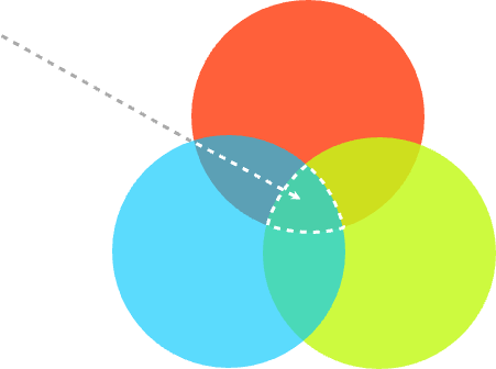 ObjectiveTruth
Literature research
Survey
Interview
ObjectiveTruth
Literature research
Survey
Interview






 Apple
Apple Tomato
 Orange


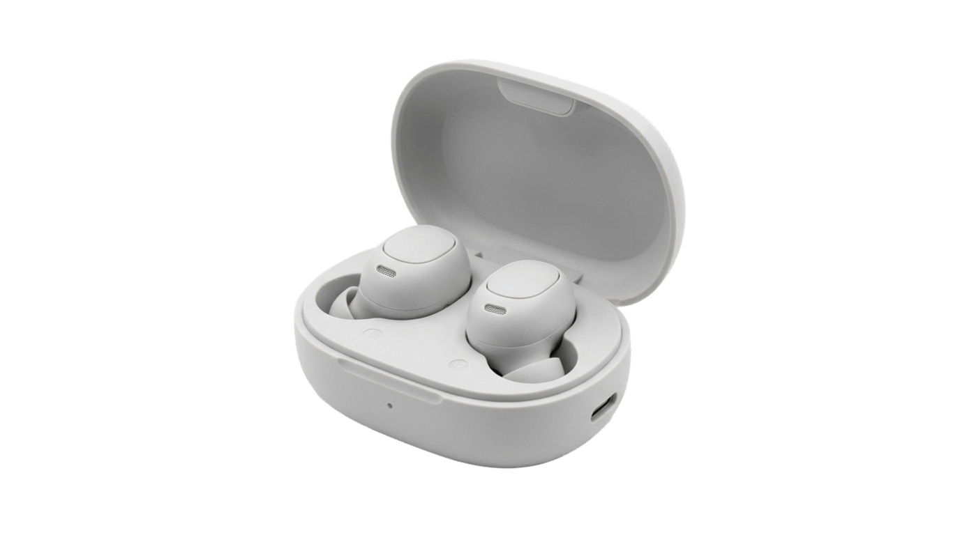
 Kiwi
Kiwi Banana
 Strawberry
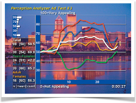

 Very satisfied
Will definitely use again
Will definitely recommend
Secure Customer
Very satisfied
Will definitely use again
Will definitely recommend
Secure Customer
 Source: Burke Inc. · http://www.burke.com/
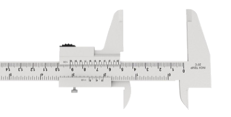



















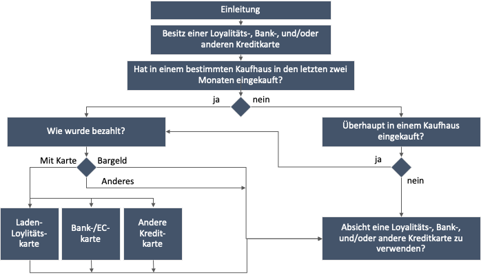
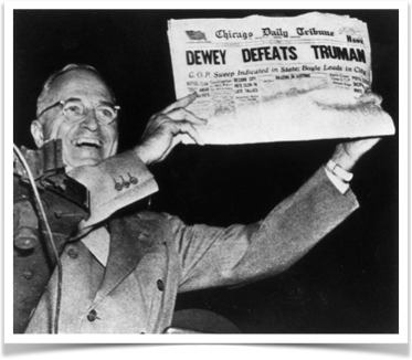


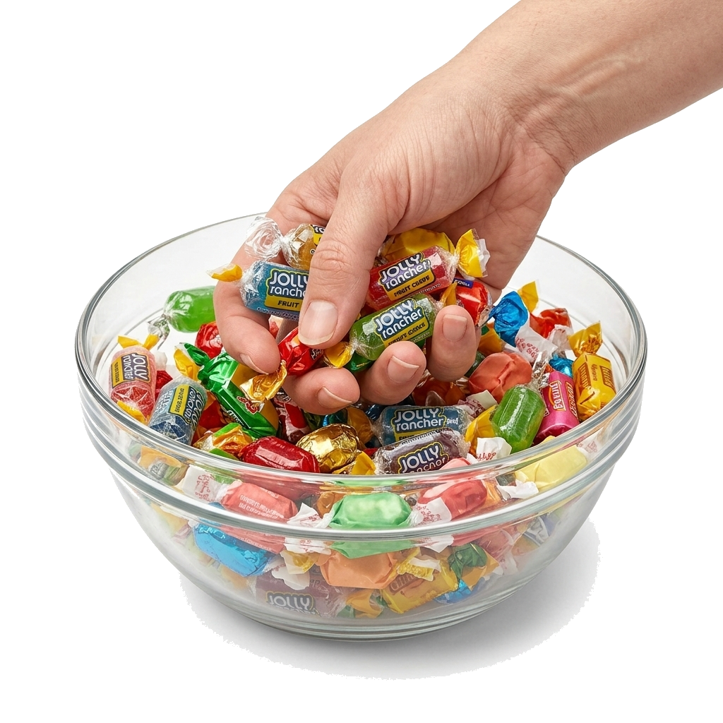








 Maximum at π = 0.5



 ncorr=n · Nn + N − 1


 for odd nfor even n





 square inches
 inches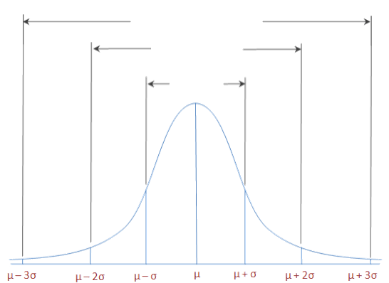






















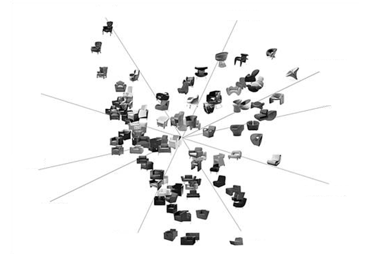
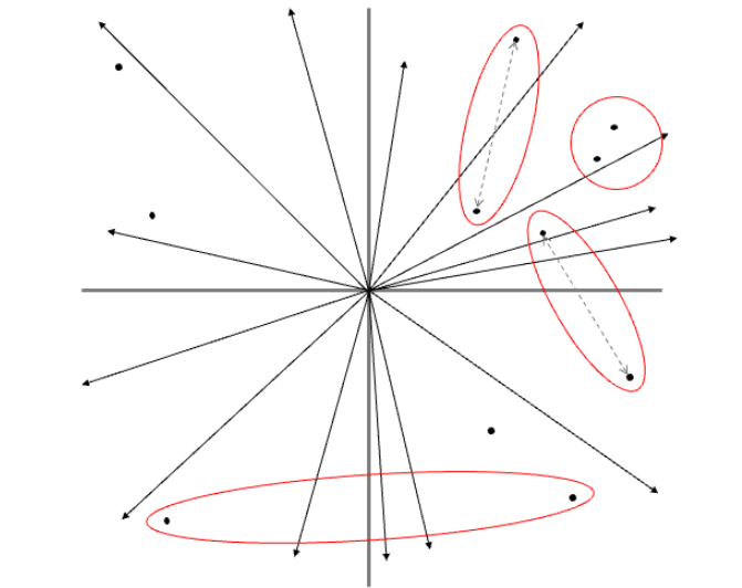
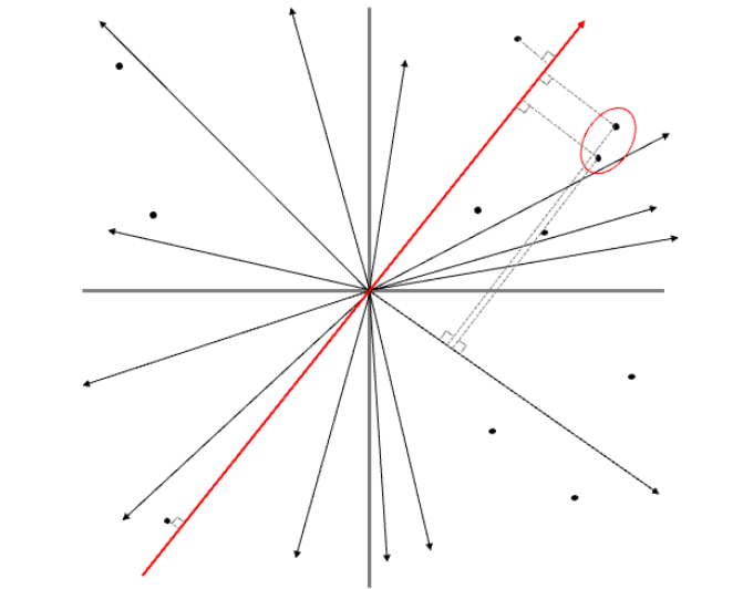
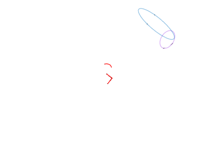
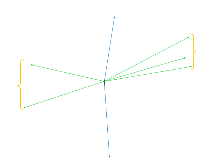
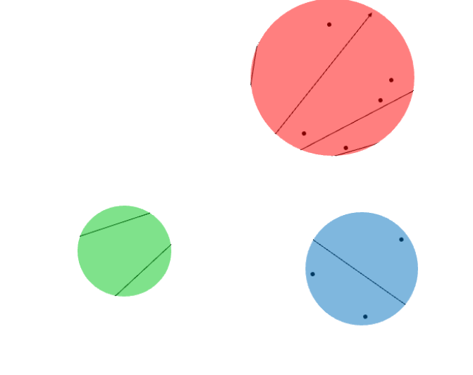

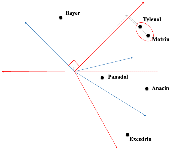
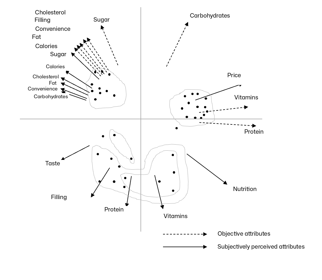
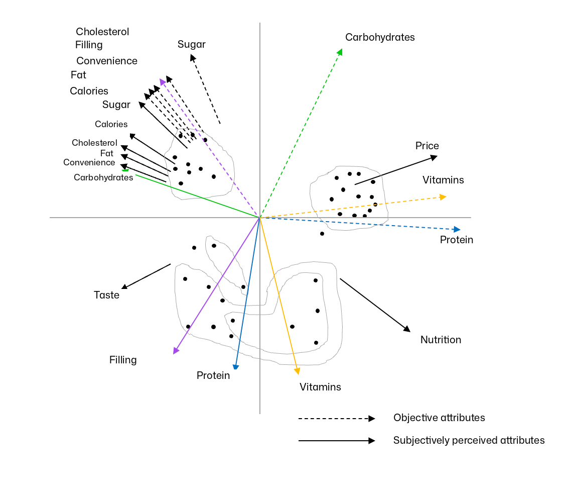




 "The readers of your reports are busy people — hardly anyone can balance report, coffee and dictionary all at once."